Solving second order ODEs using MATLAB
1. AIM
To write a program used for solving a 2nd order ODE using a function for a simple pendulum with damping and plot a graph and then show the animation of the motion of the pendulum.
2. OBJECTIVE
- To make a function for solving the 2nd order ODE.
- To make a program to show the motion of a simple pendulum with damping using the above-mentioned function.
- To make an animation showing the motion of a simple pendulum with damping.
3. METHOD
3.1 THEORY
The movement of the pendulum depends on Newton's Second Law Motion. When we write down the second law, we get a 2nd order ODE which describes the position the ball wrt time. The following equation is formed.
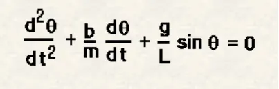
where
g = gravity(`m/s^2`)
L = length of pendulum (`m`)
m = mass of ball (`kg`)
b = damping coefficient (`Nm//s^2`)
3.2 MATLAB Program
% Motion of Simple Pendulum with damping

clear all
close all
clc

% Input parameters
b = 0.05;  % Damping coefficient (unit = Nm/s)
g = 9.81;  % Gravity (unit = m/s^2)
l = 1;     % Length of pendulum (unit = m)
m = 1;   % Mass of ball (unit = kg)

% Initial condition of Angular velocity (unit = rad/s)
theta_0 = [0;3];

% Time constraints (unit = sec)
t_span = linspace(0,20,500);

% Solution of ODE using the Function and the ode45 solver
[t, results] = ode45(@(t, theta) ode_func(t, theta, b,g,l,m), t_span, theta_0);

% Plot of the solution of ODE
% plotting displacement
plot(t,results(:,1))
hold on
% plotting velocity
plot(t,results(:,2))
title('Displacement and Velocity v/s Time')
legend('displacement','velocity')
xlabel('time (sec)')
ylabel('Angular Velocity (rad/s)')

% Plotting the motion of pendulum
% Displacement values are the values in the array results(:,1)
% Displacement values in the results array is stored in variable w
w = results(:,1);

ct=1;
for i = 1:length(w)
    u = w(i);
    x0 = 0;
    y0 = 0;
    x1 = l*sin(u)
    y1 = -l*cos(u)

    figure(2)
    plot([-1,1],[0,0])
    hold on
    plot([x0,x1],[y0,y1])
    hold on
    plot(x1,y1,'marker','o','MarkerSize',25,'MarkerFaceColor','r')
    hold off
    axis([-1.5 1.5 -1.5 1.5])
    title('Motion of Damped Pendulum')
    legend('Top base','String of length l=1m','Ball of mass m=1kg')
    pause(0.001);

    D(ct) = getframe(gcf);
    ct=ct+1;
end

movie(D)
videofile = VideoWriter('damped_pendulum_animation.avi','Uncompressed AVI');
open(videofile)
writeVideo(videofile,D)
close(videofile)
Idea behind the code:
- We start the code with clear all, close all, clc.
- Next, we define the input parameters like damping coefficient(b), gravitational force(g), length of the pendulum(l) and the mass of the ball(m).
- Then the initial condition of angular velocity and the time constraints are given.
- The function file is created for solving the ODE.
- Next, all the above inputs are put into the function file and the solution is given using the ode45 solver.
- The above solution contains two columns in which the first column has all the displacement values which are calculated and the second column has all the velocity values.
- Next, we plot a displacement and velocity v/s time graph. The hold on command is used so that both the plots are formed in one graph.
- Next, we start a for loop for finding the various positions of the ball and creating the motion of the pendulum.
- We store all the displacement values in array results(:,1) in variable w so as to simplify the code.
- In the for loop, we first start with i = initial and final values for which the loop will run.
- Then we put in the co-ordinates for the fixed end of the pendulum.
- Then we use the values of i in w for calculating every position of the ball.
- Now for showing the motion of the pendulum first we plot a line that will act as the fixed upper base.
- Then we plot the fixed point of the pendulum on this fixed point.
- Now we plot the pendulum motion and use the hold on command to plot the ball in the same graph.
- The ball is plotted using the marker command and we can decide the shape, increase the size and choose a colour for the ball.
- The hold off command is then entered to avoid creating various instances of the placement of the ball.
- A counter is entered at the beginning of the for loop and then inside the loop, its value is incremented by 1.
- Then we use D(ct) for storing all the individual frames using the getframe(gcf) command.
- Now the command movie(D) is used to create a movie and then a video file is created to dump all the frames captured in D using the videofile = VideoWriter('filename.avi','profile').
- Once the file is created it's opened using the open(videofile) command.
- Then we write all the frames captured in D to the videofile and then close the video file using the close(videofile) command.
3.3 MATLAB Function used
% Function required for solving the ODE

function [dtheta_dt] = ode_func(t,theta,b,g,l,m)

theta1 = theta(1);
theta2 = theta(2);

dtheta1_dt = theta2;
dtheta2_dt = -(((b/m)*theta2) + ((g/l)*sin(theta1)));

dtheta_dt = [dtheta1_dt; dtheta2_dt];

end- Function made is ode_ func() and is stored in the array [dthets_dt]
- The above function is used to solve the equation `d^2theta//dt^2 + b/m *d theta//dt + g/L sintheta = 0`
- Since the code is a 2nd order ODE we use theta1 and theta2 for simplifying the equation by substituting.
- `d theta1//dt = theta2`
- `d theta2//dt = -[(b/m*theta2) + (g/l*sintheta1)]`
- This way we form the function.
3.4 ode45 solver
[t, results] = ode45(@(t, theta) ode_func(t, theta, b,g,l,m), t_span, theta_0)- ode45 is a function in MATLAB that solves ODE or PDE using a numerical method which is the Runge-Kutta method.
- ode45 works by taking in the inputs which are the function to be integrated, time span, and the initial conditions.
- The proper syntax of ode45 and the inputs taken for this code is shown above.
- [t, results] is the solution array
- (t, theta) are the necessary inputs required in the function ode_func(t, theta, b,g,l,m)
- t_span is the time span.
- theta_0 is the initial condition.
3.5 ERRORS occured
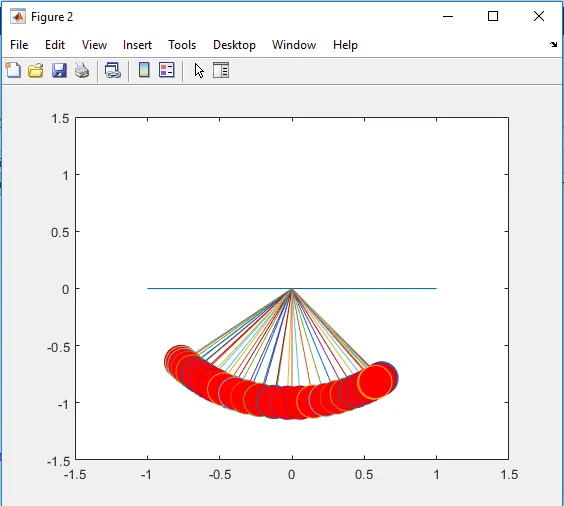
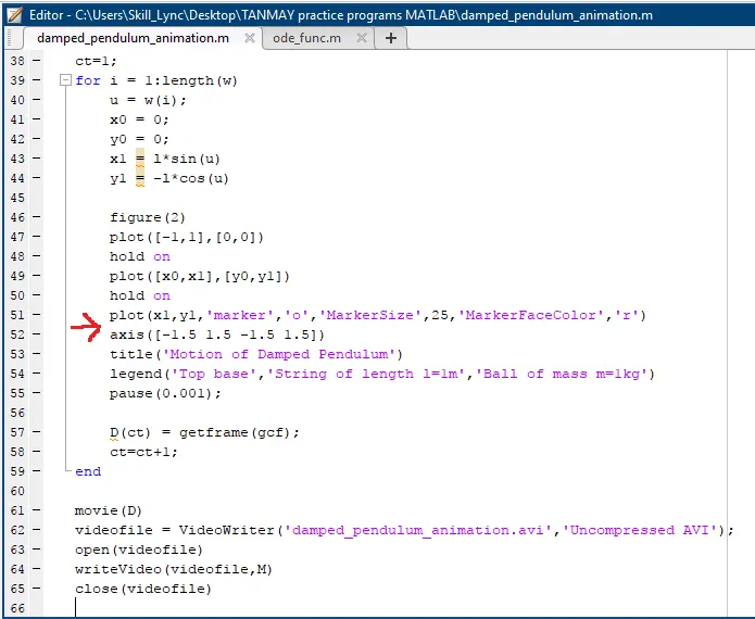 |
This error occured because I forgot to put in the hold off command. Because of this the program was plotting each and every position of the ball and displaying it. Solution Insert the hold off command. |
 |
4. LEARNING OUTCOME
- Learned how to use the function.
- Learned how to solve 2nd order ODE using the ode45 solver.
- Learned how the motion of pendulum is formed.
- Learned how to create a movie using MATLAB.
5. RESULT
The solution of the ODE is plotted which means the displacement and velocity and plotted on the angular velocity v/s time graph.
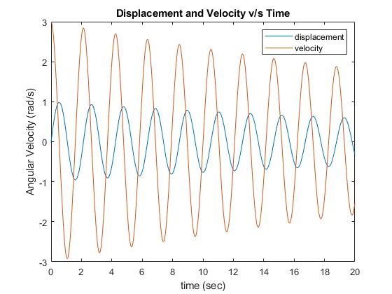
The video showing the animation of the motion of the pendulum is given below
6. CONCLUSION
For solving the ODE we need to use the ode45 solver along with the function. And due to damping the Simple pendulum will eventually come to a stop.