Week 9 - FVM Literature Review

The finite volume method (FVM) is a method for representing and evaluating partial differential equations in the form of algebraic equations. In the finite volume method, volume integrals in a partial differential equation that contain a divergence term are converted to surface integrals, using the divergence theorem. These terms are then evaluated as fluxes at the surfaces of each finite volume. Because the flux entering a given volume is identical to that leaving the adjacent volume, these methods are conservative. Another advantage of the finite volume method is that it is easily formulated to allow for unstructured meshes. The method is used in many computational fluid dynamics packages. "Finite volume" refers to the small volume surrounding each node point on a mesh.

Finite volume methods can be compared and contrasted with the finite difference methods, which approximate derivatives using nodal values, or finite element methods, which create local approximations of a solution using local data, and construct a global approximation by stitching them together. In contrast a finite volume method evaluates exact expressions for the average value of the solution over some volume, and uses this data to construct approximations of the solution within cells.

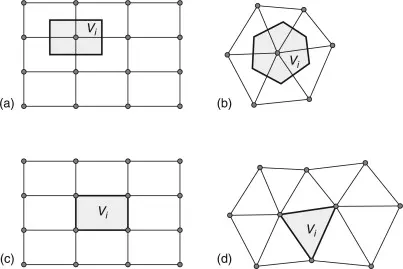
Fig 1. Mesh and dual mesh in vertex-centred FVM (a, b) and cell-centred FVM (c, d). Control volumes are defined by the grey- coloured areas.

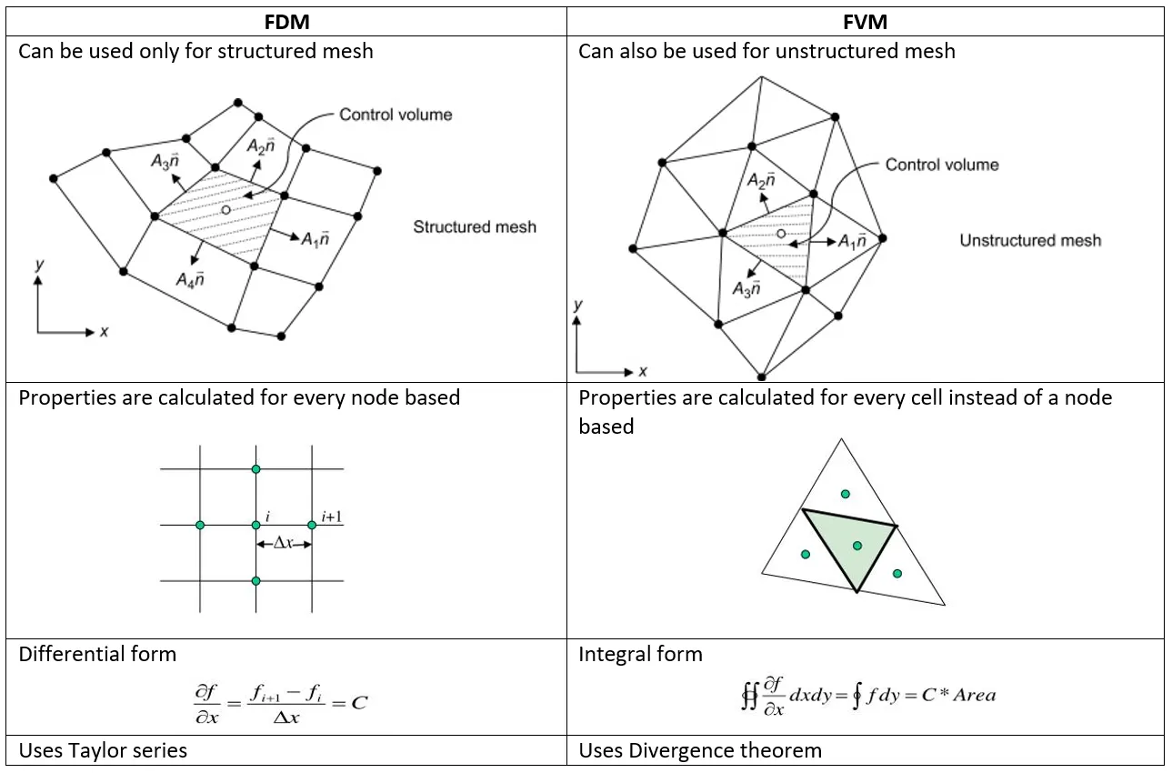
Finite difference Method (FDM)	Finite Volume Method (FVM)
The finite-difference method is the most direct approach to discretizing partial differential equations. You consider a point in space where you take the continuum representation of the equations and replace it with a set of discrete equations, called finite-difference equations.	The finite-volume method is similar to the finite-element method in that the CAD model is first divided into very small but finite-sized elements of geometrically simple shapes.
The finite-difference method is typically defined on a regular grid and this fact can be used for very efficient solution methods.	The finite-volume method is very different from the finite-element method, beginning with the concept of elements, which are instead referred to as cells.
The method is therefore not usually used for irregular CAD geometries, but more often for rectangular or block-shaped models.	The finite-volume method is based on the fact that many physical laws are conservation laws—what goes into one cell on one side needs to leave the same cell on another side.

Interpolation schemes:

The approximations of surface and volume integrals require values of the variable at location other than the computational nodes of the control volume. Values at these locations are obtained using interpolation formulae.

Linear interpolation (CDS)

Approximate values of the variable at the control volume face centre by the linear interpolation of the values at the two nearest computational nodes.

By looking the figure below, the face values appearing in the convective flux can be
computed as follows,

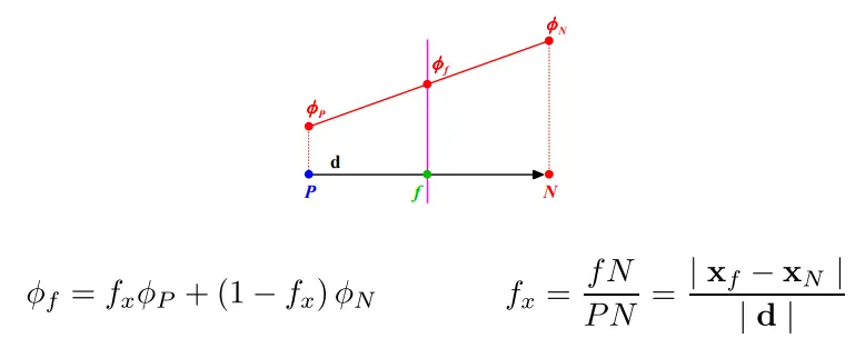
This type of interpolation scheme is known as linear interpolation or central
differencing and it is second order accurate.
However, it may generate oscillatory solutions (unbounded solutions).

It is said to be equivalent because both these methods are of order of accuracy 2.

Advantages:

• Approximation of gradients has second order of accuracy on uniform grids
• Its formally of first order on non-uniform grids.

Disadvantages:

• It may produce oscillatory solutions in case of large grid space.

Upwind Interpolation (UDS):

As the name indicates that we use the node in the upwind or upstreame of the given node.

It is used in case of convection dominated problems.

The upwind interpolation for approximating the value of a variable f at the east face of a control volume is given by

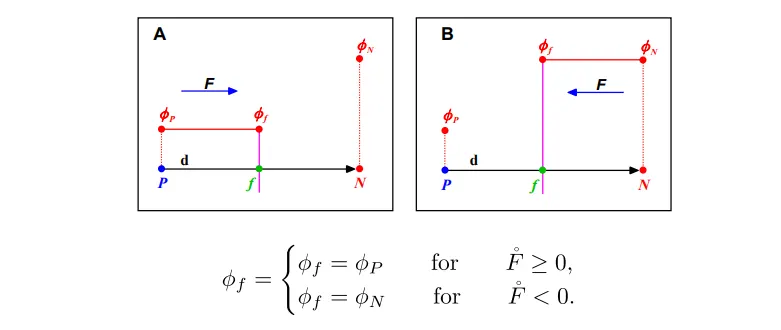
As shown in the figure above This type of interpolation scheme is known as upwind differencing and it is first order
accurate.This scheme is bounded (non-oscillatory) and diffusive.

It is said to be equivalent because all these three methods are of order of accuracy 1.

Advantages:

• UDS is the only approximation that satisfies boundedness criterion unconditionally irrespective of velocity and grid spacing i.e. never yield oscillatory solutions.

Disadvantages:

• UDS is numerically diffusive

Numerical diffusion is magnified in multi-dimensional problems if flow is oblique to the grid.

Peaks or rapid variations in the variables will be smeared out.

• Only first order accurate. Hence very fine grids are required to obtain accurate solutions.

Quadratic Upwind Interpolation for convective kinematics (QUICK):

It approximates the values of the variable at the CV face centre by Quadratic Interpolation of the values at three nearest computational nodes (1 Down stream node D & 2 Up stream nodes U , UU).

Quadratic - As it uses 3 nodes

Upwind - As it uses two upstreams

Convective Kinematics - As it is used for convective domain problems

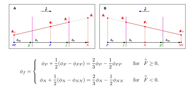
This type of interpolation scheme is known as second order upwind differencing
(SOU), linear upwind differencing (LUD) or Beam-Warming (BW), and it is second
order accurate.
For highly convective flows or in the presence of strong gradients, this scheme is
oscillatory (unbounded).

To prevent oscillations in the SOU, we add a gradient or slope limiter function .`psi(r)`

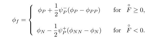
When the limiter detects strong gradients or changes in slope, it switches locally to
low resolution (upwind).

Advantages:

• It is the better version of UDS and CDS because it is more accurate than UDS and more damping in nature than CDS as it uses 3 nodes to solve.
• It is of 3rd order accurate.

Disadvantages:

• The use of QUICK can lead to subtle problems caused by such unbounded results.
• Implementation of boundary conditions can be problematic with such higher-order schemes

Total variation diminishing scheme (TVD):

A TVD scheme, is a second order accurate scheme that does not create new local undershoots and/or
overshoots in the solution or amplify existing extremes (high resolution).
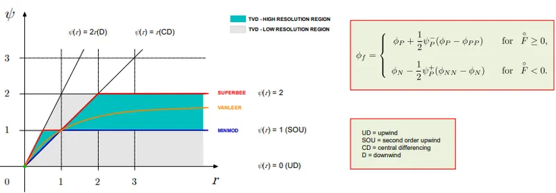
• The choice of the limiter function `psi(r)`dictates the order of the scheme and its boundedness. High resolution
schemes falls in the blue area and low resolution schemes falls in the grey area.
• The drawback of the limiters is that they reduce the accuracy of the scheme locally to first order, when`r<=0`
(sharp gradient, opposite slopes). However, this is justify when it serves to suppress oscillations.
• The various limiters have different switching characteristics and are selected according to the particular
problem and solution scheme. No particular limiter has been found to work well for all problems, and a
particular choice is usually made on a trial and error basis.
• The Sweby diagram (Sweby, 1984), gives the necessary and sufficient conditions for a scheme to be TVD.

Flux Limiter:

Flux limiters are used in high resolution schemes – numerical schemes used to solve problems in science and engineering, particularly fluid dynamics, described by partial differential equations (PDEs). They are used in high resolution schemes, such as the MUSCL scheme, to avoid the spurious oscillations (wiggles) that would otherwise occur with high order spatial discretization schemes due to shocks, discontinuities or sharp changes in the solution domain. Use of flux limiters, together with an appropriate high resolution scheme, make the solutions total variation diminishing (TVD).

Note that flux limiters are also referred to as slope limiters because they both have the same mathematical form, and both have the effect of limiting the solution gradient near shocks or discontinuities. In general, the term flux limiter is used when the limiter acts on system fluxes, and slope limiter is used when the limiter acts on system states (like pressure, velocity etc.).

They are used in high resolution schemes for solving problems described by PDEs and only come into operation when sharp wave fronts are present. For smoothly changing waves, the flux limiters do not operate and the spatial derivatives can be represented by higher order approximations without introducing spurious oscillations.

`(du_i)/(dt)+1/(Deltax_i)[F(u_(i+1/2))-F(u_(i-1/2))]=0`

where,`F(u_(i+1/2))`and `F(u_(i-1/2))``represent edge fluxes for the ith cell. If these edge fluxes can be represented by low and high resolution schemes, then a flux limiter can switch between these schemes depending upon the gradients close to the particular cell, as follows,`

`F(u_(i+1/2))=f_(i+1/2)^(low)-phi(r_i)(f_(i+1/2)^(low)-f_(i+1/2)^(high))`

`F(u_(i-1/2))=f_(i-1/2)^(low)-phi(r_i)(f_(i-1/2)^(low)-f_(i-1/2)^(high))`

where

`f^(low)`=low resolution flux

`f^(high)`=high resolution flux

`phi(r)`= flux limiter function