Week 5 - Rayleigh Taylor Instability

ABSTRACT

some practical CFD models that have been based on the mathematical analysis of Rayleigh Taylor waves and how these mathematical models have been adapted for CFD calculations. Performing the Rayleigh Taylor instability simulation for 2 different mesh sizes with the base mesh being 0.5 mm. Compare the results by showing the animations. Observing the differences in the animation and explain the effect of mesh size on simulation. Running one more simulation with water and user-defined material(density = 400 kg/m³, viscosity = 0.001 kg/m-s) for refined mesh and Defining Atwood Number. Finding out the Atwood number for both the cases and explaining how the variation in Atwood number in the above two cases affects the behavior of the instability.

Case 1: What are some practical CFD models that have been based on the mathematical analysis of Rayleigh Taylor waves? In your own words, explain how these mathematical models have been adapted for CFD calculations.

In CFD, currently there are two approaches for the numerical calculation of multiphase flows: the Euler-Lagrange approach and the Euler-Euler approach.

Euler-Lagrange approach

The Lagrangian discrete phase model follows the Euler-Lagrange approach. The fluid phase is treated as a continuum by solving the Navier-Stokes equations, while the dispersed phase is solved by tracking a large number of particles, bubbles, or droplets through the calculated flow field. The dispersed phase can exchange momentum, mass, and energy with the fluid phase.

The E-L approach offers advantages such as providing full information on particle trajectories and local residence time, handling a distribution of particle sizes and predicting differences in local particle velocities; particle-particle collisions and particle-wall interactions can also be handled realistically, albeit at increased computational expense.

Simulation of multiphase flow by the E-L method solves the fluid phase as a continuum and the dispersed phase as a discrete phase within a Langrangian framework by resolving the force balance on each numerical particle.

Governing equations for E-L model:

Equations of particle motion:

In Lagrangian coordinates, particle position and momentum equa-tion for the dispersed phase are exploited, respectively, as:
`((d_x)_pi)/dt=(u_p)_pi`

and

`((d_u)_pi)/dt=Sigma_(i=n)^n+(1-(m_pi)/m_L)g`

where, 'i' is the particle index within a population of 'n' particles; `x_pi,u_pi andm_pi` are the ith particle position, velocity and mass, respectively; 't' is time; `m_L` is the mass of liquid displaced by the particle and 'g' represents gravitational acceleration;`(1-(m_pi)/m_L)g` is the apparent weight of a particle per unit mass expressing the effect of buyoancy; Fp represents the sum of all forces acting on a particle, including Brownian, Saffman lift, viscous drag, added mass, pressure gradient, thermophoretic and Basset acceleration. For the system studied here, the Brownian and Saffman lift forces are irrelevant since the particles considered are well above the submicron and micron scales. In addition, the pressure gradient force is negligible because the density of the glass particles used is much higher than that of the suspending liquid, and so is the thermophoretic force because of the absence of a significant temperature gradient. The Basset force is also insignificant as there is no sharp acceleration in the flow studied and, hence, the only contributions to `F_p` arise from the total drag and added mass force.

Particle-particle collision model:

Particle-particle collisions play a significant role in non-dilute suspension flows, and need to be taken into consideration. In the stochastic inter-particle collision model proposed by Sommerfeld (2001), collision partners are fictitious and collision probability is calculated according to kinetic theory. Based on the local size and velocity distributions of the dispersed phase, the stochastic collision model creates a fictitious collision partner. Consequently, the fictitious particle represents the population of local particles. So, it is not necessary to determine whether a collision occurs by knowing the locations of nearby real particles or by looking for collision partners. For each computational element, only the particle size- and velocity-distribution functions are necessary.

A partial correlation (f) of the turbulent fluctuation velocities between a real particle and a fictitious particle, is used to calculate the instantaneous velocity of the fictitious particle`u_(fict)^29`The correlation is a function of the turbulent Stokes number (`St_t`) which is a ratio of the relaxation time `tau_R=(rho_pd^2)/(18mu)`to the eddy life time `tau_e=0.3k/epsilon`.

`f(St_t)=e^(-0.55(tau_r/tau_e)^0.4)`

Thus, the fluctuating velocity `u'_(fict)` of the fictitious collision partner can be expressed as:

`u'_(fict.j)=f(St_t)u'_(real.j)+sigma_(p.j)sqrt(1-f(St_t)^2xi`

where, the index j denotes the three coordinate directions,`sigma_(p.j)` is a mean fluctuation velocity of the `j^(th)` component in the control volume, and `xi` represents the uncorrelated portion of the fluctuation velocity of the fictitious particle.

The resulting post-collision velocity (`u_p^**` ) of the real particle is then estimated using the
coeficient of restitution (ε), thus

`u_p^**=u_p(1-(1+epsilon)/(1+m_(real)/m_(fict)))`

where, `m_(real)` and `m_(fict)` are the masses of the real and fictitious particles,
respectively.

Liquid phase modelling:

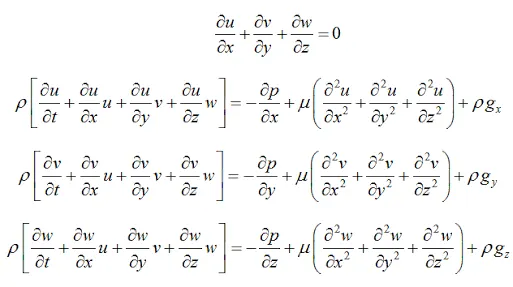
In the E-L method, the carrier liquid is treated as a continuum by solving the 3D system of Navier Stokes equations, including the continuity equation:

Euler-Euler Approach

In Fluent three different Euler-Euler multiphase models are available:

• Volume of fluid (VOF) model
• Mixture model
• Eulerian model

The VOF Model

The VOF model is a surface-tracking technique applied to a fixed Eulerian mesh. It is designed for two or more immiscible fluids where the position of the interface between the fluids is of interest.

In computational fluid dynamics, the volume of fluid (VOF) method is a free-surface modelling technique, i.e. a numerical technique for tracking and locating the free surface (or fluid–fluid interface). It belongs to the class of Eulerian methods which are characterized by a mesh that is either stationary or is moving in a certain prescribed manner to accommodate the evolving shape of the interface. As such, VOF is an advection scheme—a numerical recipe that allows the programmer to track the shape and position of the interface, but it is not a standalone flow solving algorithm. The Navier–Stokes equations describing the motion of the flow have to be solved separately. The same applies for all other advection algorithms.

Illustration of fluid using VOF Model.

The Mixture Model

The mixture model is designed for two or more phases (fluid or particulate). As in the Eulerian model, the phases are treated as interpenetrating continua. It can be used to model multiphase flows where the phases move at different velocities, but assume local equilibrium over short spatial length scales. It can be used to model homogeneous multiphase flows with very strong coupling and phases moving at the same velocity and lastly, the mixture models are used to calculate non-Newtonian viscosity.

The mixture model can model phases (fluid or particulate) by solving the momentum, continuity, and energy equations for the mixture, the volume fraction equations for the secondary phases, and algebraic expressions for the relative velocities. Typical applications include sedimentation, cyclone separators, particle-laden flows with low loading, and bubbly flows where the gas volume fraction remains low.

The mixture model is a good substitute for the full Eulerian multiphase model in several cases. A full multiphase model may not be feasible when there is a wide distribution of the particulate phase or when the interphase laws are unknown or their reliability can be questioned. A simpler model like the mixture model can perform as well as a full multiphase model while solving a smaller number of variables than the full multiphase model.

The mixture model allows you to select granular phases and calculates all properties of the granular phases. This is applicable for liquid-solid flows.[1].

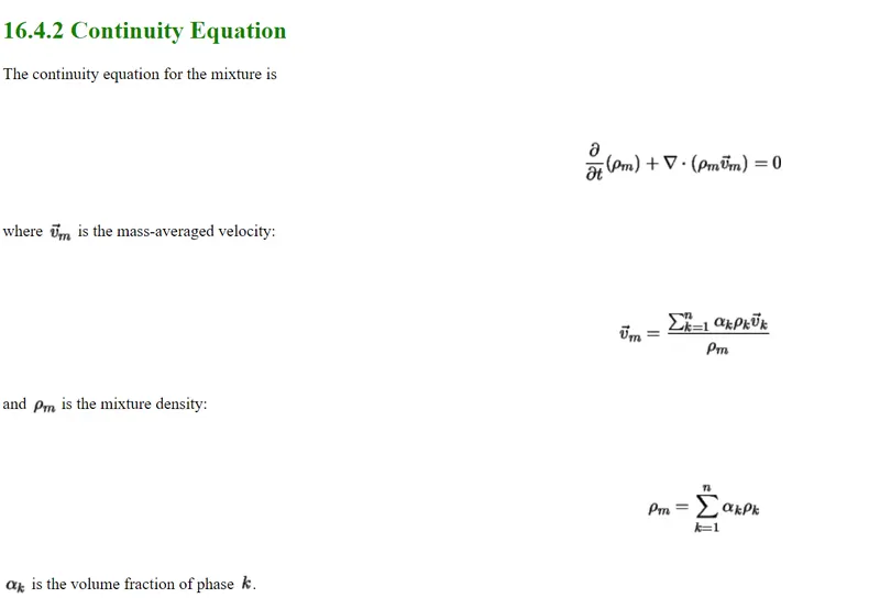
Continuity Equations:

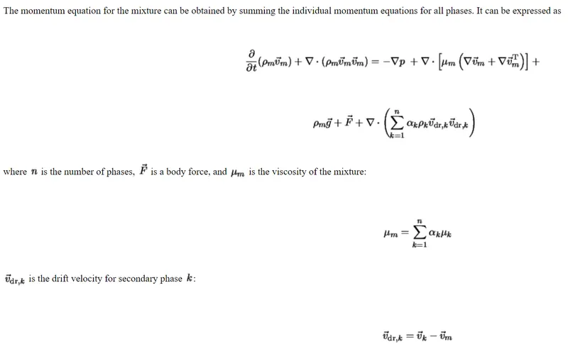
Momentum Equations:

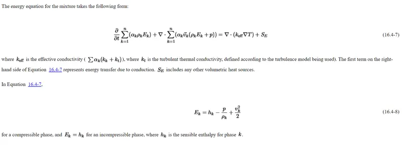
Energy Equations:

The Eulerian Model

The Eulerian model is the most complex of the multiphase models in. It solves a set of momentum and continuity equations for each phase.

The Eulerian multiphase model in ANSYS FLUENT allows for the modeling of multiple separate, yet interacting phases. The phases can be liquids, gases, or solids in nearly any combination. An Eulerian treatment is used for each phase, in contrast to the Eulerian-Lagrangian treatment that is used for the discrete phase model.

With the Eulerian multiphase model, the number of secondary phases is limited only by memory requirements and convergence behavior. Any number of secondary phases can be modeled, provided that sufficient memory is available. For complex multiphase flows, however, you may find that your solution is limited by convergence behavior. See this section in the separate User's Guide for multiphase modeling strategies.

ANSYS FLUENT's Eulerian multiphase model does not distinguish between fluid-fluid and fluid-solid (granular) multiphase flows. A granular flow is simply one that involves at least one phase that has been designated as a granular phase.

The ANSYS FLUENT solution is based on the following:

• A single pressure is shared by all phases.
• Momentum and continuity equations are solved for each phase.
  • Granular temperature (solids fluctuating energy) can be calculated for each solid phase. You can select either an algebraic formulation, a constant, a user-defined function, or a partial differential equation.
  • Solid-phase shear and bulk viscosities are obtained by applying kinetic theory to granular flows. Frictional viscosity for modeling granular flow is also available. You can select appropriate models and user-defined functions for all properties. The following parameters are available for granular phases:
• Several interphase drag coefficient functions are available, which are appropriate for various types of multiphase regimes. (You can also modify the interphase drag coefficient through user-defined functions, as described in the separate UDF Manual.)
• All of the - turbulence models are available, and may apply to all phases or to the mixture.[2]

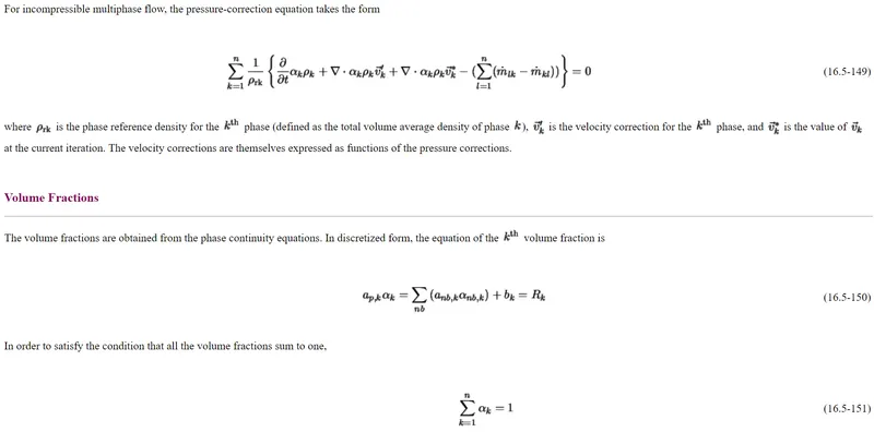
Case 2: Perform the Rayleigh Taylor instability simulation for 2 different mesh sizes with the base mesh being 0.5 mm. Compare the results by showing the animations( Attach them from your google drive). Observe the differences in the animation and explain the effect of mesh size on simulation. Also, explain why a steady-state approach might not be suitable for these types of simulation.

In this case we have to create the two 2-D square geometry with 20 mm for both upward and downward in spaceclaim as shown in the figure below. Then with the help of esxtrude option we have to create a surface area for the geometry. After creating the surafce of the geometry in the workbench we have to share the two surafce of the geometry by using force share and selecting the geometry, after selecting the geometry click in share to share the surface and automatically the topology of the surface will also get shared in it. Now our geometry has been created.

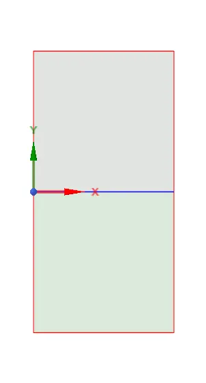
Sharing of topology.

Part A) Meshing size of 0.5mm

Now changing the mesh size to 0.5mm and changing the state to the transient form and applying the gravity in neagtive y-direction and changing the function to implicit.

After doing all this initializing it and patching it in phase 2 in voume fraction by keeping the air value 0 and water value 1.

Now running the calculation for 200 number of tiem step with time step size as 0.005. After completion of the calculation we will be getting the contour and the residual chart as shown below:

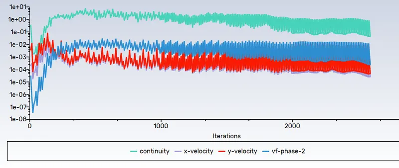
Video link for the contour:

Animation for case 1

Part B) Meshing size of 0.3mm

Now changing the mesh size to 0.3mm and changing the state to the transient form and applying the gravity in neagtive y-direction and changing the function to implicit.

After doing all this initializing it and patching it in phase 2 in voume fraction by keeping the air value 0 and water value 1.

Now running the calculation for 200 number of tiem step with time step size as 0.005. After completion of the calculation we will be getting the contour and the residual chart as shown below:

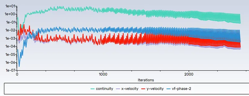
Video link for the contour:

Animation for case 2

After observing the both contours we can say that the mesh size with high element size tells us the understanding of the flow of both the fluids till the fluids settles down. And it also tells the flow of fluids in detail with respect to gravity.

The steady state appraoch is not suitable because the flow is transient flow and the paramters change with respect to the time where as in this case the steadt state flow is not possible so transient flow is the best.

Case 3) Run one more simulation with water and user-defined material(density = 400 kg/m³, viscosity = 0.001 kg/m-s) for refined mesh.

Taking mesh size as 0.5mm.

It is as similar to the previous case but we need to change the material to user defined and water as mention in the requirements after doing this follow the previous steps for running the calculations.

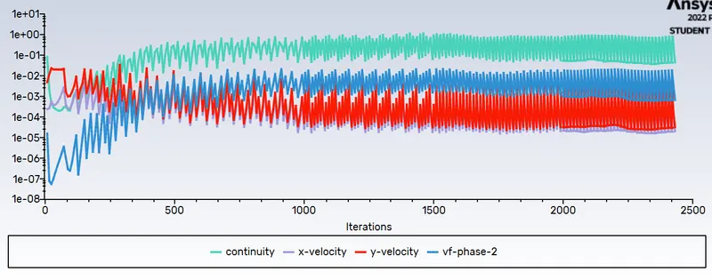
The residual:

Video link for the contour:

Animation for user-defined simulation

Case 4) Define the Atwood Number. Find out the Atwood number for both the cases and explain how the variation in Atwood number in the above two cases affects the behavior of the instability.

Atwood Number:

The Atwood number (A) is a dimensionless number in fluid dynamics used in the study of hydrodynamic instabilities in density stratified flows. It is a dimensionless density ratio defined as:

`A = (rho_1 - rho_2)/(rho_1+rho_2)`

Where, `rho_1` - density of Heavier Fluid

`rho_2` - density of lighter fluid

Atwood number is an important parameter in the study of Rayleigh–Taylor instability and Richtmyer–Meshkov instability. In Rayleigh–Taylor instability, the penetration distance of heavy fluid bubbles into the light fluid is a function of acceleration time scale,`Ag(t)^2` where g is the gravitational acceleration and t is the time.

A)

Density of air=1.225 kg/m^3=`rho_2`

Density of water= 998.2 kg/m^3=`rho_1`

A=`(rho_1-rho_2)/(rho_1+rho_2)`=998.2-1.225/998.2+1.225

A=0.997

B)

Density of user-defined material= 400 kg/m^3=`rho_2`

Density of water= 998.2 kg/m^3=`rho_1`

A=`(rho_1-rho_2)/(rho_1+rho_2)`=998.2-400/998.2+400

A=0.427

Conclusion:

SO we can conclude that

• Higher the atwood Number the Instabilites are sudden and Reach steady state more rapidly
• Lower the Atwood Number Instabilites Take time and Reach steady state slowly
• From the animation video it is able to visualize the RT instability of two fluid accurately. It is also concluded that fine meshing provide a clear picture of simulation as compared to baselinemeshing.

RTI evolves in three distinct stages:

• Linear stability,
• mushroom head(falling) or bubble(rising) formation,
• long term evolution due to bubble merging and mixing.

For low Atwood number, bubble and mushroom head shape is relatively symmetrical, the disturbances or perturbations are linear for a larger time.

for large Atwood number, bubble and mushroom head shape is less symmetrical, also it occurs very rapidly at an accelerating rate which leads to a nonlinear growth rate.

• Since the simulation involves capturing instabilities that are changing in an unpredictable manner as a function of time, the transient approach is preferred over the steady-state approach.

References:

[1]:https://www.afs.enea.it/project/neptunius/docs/fluent/html/th/node308.htm

[2]:https://www.afs.enea.it/project/neptunius/docs/fluent/html/th/node319.htm