Week 11 - Simulation of Flow through a pipe in OpenFoam
We have to simulate an axisymmetric flow by applying the wedge boundary condition. The flow is laminar and flows through a constant cross-section pipe at an inlet Reynold's number of 2100.
To do a transient or steady state simulation and you will validate your results with the Hagen- Poiseuille's equations for the fully developed flow.
After this writing the code in Matlab to automate the generation of blockMeshDict file. The code should take inputs like pipe length, diameter, wedge angle, etc and output a fully functional blockMeshDict file.
Fluid flow describes how fluid behaves when in motion. It is a vital engineering perspective and studied in hydraulics and fluid mechanics. The theory of fluid flow is very important for effectively sizing piping and equipment.
ny substance which can flow is called fluid. Liquids, gases, or a mixture of both of them are collectively called fluids. They contain a finite mass, occupy a space, and are tangible. They are substances which either made up of different molecules or particles. They are flowing when the particles of the substance have a change in the relative position concerning time. The properties acquired by the fluids are
- It does have a mass of its own.
- It doesn’t have shapes.
- It occupies the shape of the vessel or pipe where it is flowing.
- It can flow under its weight.
Mechanics is the study of force and its effects. The forces that act on the fluid are
- Surface force
- Body force ( gravitational force)
Flow through the pipes
Flow-through pipes or fluid flow is a type of flow within a closed conduit with a certain pressure. Another type of flow is an open channel flow. These fluid flows are applied to transport chemicals, petroleum products, gas products, sewage flows, household water supply, etc. in different piping and pipeline systems.
The flow of all Real fluids is termed viscous flow( as they possess a viscosity) These properties of viscosity are characterized by the shear stresses or the frictional forces between the fluid layers and fluid to a solid surface, same as the physical parameters of the pipe & the external force’s affecting the piping system by displacement and loads. The fluid’s flowing and the flow parameters affect the piping system in many ways.
The types of the flow:
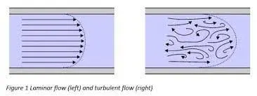
Laminar Flow:
When the fluid moves slowly in layers in a pipe, without much mixing among the layers. usually occurs when the velocity is low / the fluid is very viscous. The maximum flow will be at the center of the pipes and the minimum flow at the pipe walls.
Where the Reynolds number is less than 2300 laminar flow will occur and the resistance to flow will be independent of the pipe wall roughness. The friction factor for laminar flow can be calculated from 64 / Re
Turbulent Flow:
When the velocity of the flow exceeds some threshold value for a given fluid in a pipe, ie. when the velocity is high. flow becomes turbulent, the fluid becomes irregularly fluctuating with time. Velocity at the center of the pipe is approximately equal to the average flow velocity.
Turbulent flow occurs when the Reynolds number exceeds 4000.
| Reynold's Number | Conditions of law |
| Re<2000 | Laminar |
| 2000<Re<4000 | Transitional |
| Re>4000 | Turbulent |
Eddy currents are present within the flow and the ratio of the internal roughness of the pipe to the internal diameter of the pipe needs to be considered to be able to determine the friction factor. In large diameter pipes the overall effect of the eddy currents is less significant. In small diameter pipes the internal roughness can have a major influence on the friction factor.
Reynolds Number:
The Reynolds number is the ratio of inertial forces to viscous forces within a fluid that is subjected to relative internal movement due to different fluid velocities. A region where these forces change behavior is known as a boundary layer, such as the bounding surface in the interior of a pipe
The Reynolds number (Re) of a flowing fluid is obtained by dividing the kinematic viscosity (viscous force per unit length) into the inertia force of the fluid (velocity x diameter)
Kinematic viscosity = (dynamic viscosity)/(fluid density)
Reynolds number = (Fluid velocity x Internal pipe diameter)/(kinematic viscosity)
Hagen- Poiseuille's equations :
In nonideal fluid dynamics, the Hagen–Poiseuille equation, also known as the Hagen–Poiseuille law, Poiseuille law or Poiseuille equation, is a physical law that gives the pressure drop in an incompressible and Newtonian fluid in laminar flow flowing through a long cylindrical pipe of constant cross section. It can be successfully applied to air flow in lung alveoli, or the flow through a drinking straw or through a hypodermic needle.
The Hagen–Poiseuille equation describes the relationship between pressure, fluidic resistance and flow rate, analogous to voltage, resistance, and current, respectively, in Ohm's law for electrical circuits ( V = R I ). Both electrical resistance and fluidic resistance are proportional to the length of the device.
`Deltap=(8muLQ)/(piR^4)`
`Deltap`=pressure difference between the two ends
`mu`= dynamic viscosity
L = length of pipe
Q = Volumetric flow rate
R = pipe radius
PROGRAM CODES AND FILES :
First, we are going to write a MatLab code to automate the generation of the blockMeshDict file, which takes our respective inputs and outputs a fully functional blockMeshDict file.
The blockMeshDict file has been written automatically by the MatLab program as shown above, which we use to create the geometry of the wedge and run the simulation for the same.
% SIMULATION OF FLOW THROUGH A PIPE
% Code to automate generation of blockMeshDict file
clear all
close all
clc


% INPUTS
% Assumptions
% Diameter of Pipe (m)
D = 0.02;

% Radius of Pipe (m)
R = D/2;

% Reynold's Number
Re = 2100;

% Wedge Angle (degrees)
theta = 4;

% Total Length of the Pipe (m)
L = 2.8;


% Assuming working fluid is water at 25° C
% Density of water (kg/m³)
rho = 997;

% Dynamic Viscosity of Water (Pa.s)
mu = 8.90 * 10^-4;

% Kinematic Viscosity of Water (m^2/s)
nu = mu/rho;


% Hydrodynamic Entrance Length (m)
L_h = 0.06 * Re * D;


% HAGEN - POISEUILLE'S FLOW EQUATIONS
% Average Velocity (m/s)
V_avg = (mu * Re)/(rho * D);

% Maximum Velocity (m/s)
V_max = 2 * V_avg;

% Pressure Drop (Pa)
delta_p = (32*mu*V_avg*L)/(D^2);

% Kinematic Pressure Drop (Pa)
kinematic_delta_p = delta_p/rho;


% DEFINING THE GEOMETRY
% Vertices
V0 = [0 0 0];
V1 = [0 R*cosd(theta/2) -R*sind(theta/2)];
V2 = [0 R*cosd(theta/2) R*sind(theta/2)];

V3 = [L 0 0];
V4 = [L R*cosd(theta/2) -R*sind(theta/2)];
V5 = [L R*cosd(theta/2) R*sind(theta/2)];


% BLOCKMESHDICT FILE
% Creating the file
% Header
h1 = '/*--------------------------------*- C++ -*----------------------------------*\';
h2 = '  =========                 |';
h3 = '  \\      /  F ield         | OpenFOAM: The Open Source CFD Toolbox';
h4 = '   \\    /   O peration     | Website:  https://openfoam.org';
h5 = '    \\  /    A nd           | Version:  9';
h6 = '     \\/     M anipulation  |';
h7 = '\*---------------------------------------------------------------------------*/';
h8 = 'FoamFile';
h9 = '{';
h10 = '    format      ascii;';
h11 = '    class       dictionary;';
h12 = '    object      blockMeshDict;';
h13 = '}';
h14 = '// * * * * * * * * * * * * * * * * * * * * * * * * * * * * * * * * * * * * * //';


% Creating BlockMesh File
f1 = fopen('blockMeshDict.txt');

% Header
fprintf(f1,'%s\n',h1);
fprintf(f1,'%s\n',h2);
fprintf(f1,'%s\n',h3);
fprintf(f1,'%s\n',h4);
fprintf(f1,'%s\n',h5);
fprintf(f1,'%s\n',h6);
fprintf(f1,'%s\n',h7);
fprintf(f1,'%s\n',h8);
fprintf(f1,'%s\n',h9);
fprintf(f1,'%s\n',h10);
fprintf(f1,'%s\n',h11);
fprintf(f1,'%s\n',h12);
fprintf(f1,'%s\n',h13);
fprintf(f1,'%s\n\n',h14);

% Conversion Factor
fprintf(f1,'%s\n\n','convertToMeters 1;');

% Vertices
fprintf(f1,'%s\n','vertices');
fprintf(f1,'%s\n','(');
fprintf(f1,'\t(%d %d %d)\n',V0);
fprintf(f1,'\t(%d %f %f)\n',V1);
fprintf(f1,'\t(%d %f %f)\n',V2);
fprintf(f1,'\t(%.2f %d %d)\n',V3);
fprintf(f1,'\t(%.2f %f %f)\n',V4);
fprintf(f1,'\t(%.2f %f %f)\n',V5);
fprintf(f1,'%s\n\n',');');

% Blocks
fprintf(f1,'%s\n','blocks');
fprintf(f1,'%s\n','(');
fprintf(f1,'\thex (0 3 4 1 0 3 5 2) (50 10 1) simpleGrading (1 1 1)\n');
fprintf(f1,'%s\n\n',');');

% Edges
fprintf(f1,'%s\n','edges');
fprintf(f1,'%s\n','(');
fprintf(f1,'\tarc 2 1 (%d %.3f %d)\n',0,R,0);
fprintf(f1,'\tarc 4 5 (%.3f %.3f %d)\n',L,R,0);
fprintf(f1,'%s\n\n',');');

% Boundary
fprintf(f1,'%s\n','boundary');
fprintf(f1,'%s\n','(');

% Axis
fprintf(f1,'\taxis\n');
fprintf(f1,'\t{\n');
fprintf(f1,'\t\ttype empty;\n');
fprintf(f1,'\t\tfaces\n');
fprintf(f1,'\t\t(\n');
fprintf(f1,'\t\t\t(0 3 3 0)\n');
fprintf(f1,'\t\t);\n');
fprintf(f1,'\t}\n\n');

% Inlet
fprintf(f1,'\tinlet\n');
fprintf(f1,'\t{\n');
fprintf(f1,'\t\ttype patch;\n');
fprintf(f1,'\t\tfaces\n');
fprintf(f1,'\t\t(\n');
fprintf(f1,'\t\t\t(0 2 1 0)\n');
fprintf(f1,'\t\t);\n');
fprintf(f1,'\t}\n\n');

% Outlet
fprintf(f1,'\toutlet\n');
fprintf(f1,'\t{\n');
fprintf(f1,'\t\ttype patch;\n');
fprintf(f1,'\t\tfaces\n');
fprintf(f1,'\t\t(\n');
fprintf(f1,'\t\t\t(3 4 5 3)\n');
fprintf(f1,'\t\t);\n');
fprintf(f1,'\t}\n\n');

% Front Face
fprintf(f1,'\tfront\n');
fprintf(f1,'\t{\n');
fprintf(f1,'\t\ttype wedge;\n');
fprintf(f1,'\t\tfaces\n');
fprintf(f1,'\t\t(\n');
fprintf(f1,'\t\t\t(0 3 5 2)\n');
fprintf(f1,'\t\t);\n');
fprintf(f1,'\t}\n\n');

% Back Face
fprintf(f1,'\tback\n');
fprintf(f1,'\t{\n');
fprintf(f1,'\t\ttype wedge;\n');
fprintf(f1,'\t\tfaces\n');
fprintf(f1,'\t\t(\n');
fprintf(f1,'\t\t\t(0 1 4 3)\n');
fprintf(f1,'\t\t);\n');
fprintf(f1,'\t}\n\n');

% Top Wall
fprintf(f1,'\tpipeWall\n');
fprintf(f1,'\t{\n');
fprintf(f1,'\t\ttype wall;\n');
fprintf(f1,'\t\tfaces\n');
fprintf(f1,'\t\t(\n');
fprintf(f1,'\t\t\t(1 2 5 4)\n');
fprintf(f1,'\t\t);\n');
fprintf(f1,'\t}\n');

fprintf(f1,'%s\n\n',');');
fprintf(f1,'%s\n','mergePatchPairs');
fprintf(f1,'%s\n','(');
fprintf(f1,'%s\n\n',');');
fprintf(f1,'%s\n','// ************************************************************************* //');
After running the program the the blockMesh file have been automatically created which can paste it instead of the previous blockMesh file as shown below:
/*--------------------------------*- C++ -*----------------------------------*\
  =========                 |
  \\      /  F ield         | OpenFOAM: The Open Source CFD Toolbox
   \\    /   O peration     | Website:  https://openfoam.org
    \\  /    A nd           | Version:  9
     \\/     M anipulation  |
\*---------------------------------------------------------------------------*/
FoamFile
{
    format      ascii;
    class       dictionary;
    object      blockMeshDict;
}
// * * * * * * * * * * * * * * * * * * * * * * * * * * * * * * * * * * * * * //

convertToMeters 1;

vertices
(
	(0 0 0)
	(0 0.009994 -0.000349)
	(0 0.009994 0.000349)
	(2.80 0 0)
	(2.80 0.009994 -0.000349)
	(2.80 0.009994 0.000349)
);

blocks
(
	hex (0 3 4 1 0 3 5 2) (50 10 1) simpleGrading (1 1 1)
);

edges
(
	arc 2 1 (0 0.010 0)
	arc 4 5 (2.800 0.010 0)
);

boundary
(
	axis
	{
		type empty;
		faces
		(
			(0 3 3 0)
		);
	}

	inlet
	{
		type patch;
		faces
		(
			(0 2 1 0)
		);
	}

	outlet
	{
		type patch;
		faces
		(
			(3 4 5 3)
		);
	}

	front
	{
		type wedge;
		faces
		(
			(0 3 5 2)
		);
	}

	back
	{
		type wedge;
		faces
		(
			(0 1 4 3)
		);
	}

	pipeWall
	{
		type wall;
		faces
		(
			(1 2 5 4)
		);
	}
);

mergePatchPairs
(
);

// ************************************************************************* //
ControlDict File:
Changing the values of the directory as per the requirements.
/*--------------------------------*- C++ -*----------------------------------*\
  =========                 |
  \\      /  F ield         | OpenFOAM: The Open Source CFD Toolbox
   \\    /   O peration     | Website:  https://openfoam.org
    \\  /    A nd           | Version:  10
     \\/     M anipulation  |
\*---------------------------------------------------------------------------*/
FoamFile
{
    format      ascii;
    class       dictionary;
    location    "system";
    object      controlDict;
}
// * * * * * * * * * * * * * * * * * * * * * * * * * * * * * * * * * * * * * //

application     icoFoam;

startFrom       startTime;

startTime       0;

stopAt          endTime;

endTime         5;

deltaT          0.001;

writeControl    timeStep;

writeInterval   20;

purgeWrite      0;

writeFormat     ascii;

writePrecision  6;

writeCompression off;

timeFormat      general;

timePrecision   6;

runTimeModifiable true;


// ************************************************************************* //
p File:
Changing the values of the pressure file.
/*--------------------------------*- C++ -*----------------------------------*\
  =========                 |
  \\      /  F ield         | OpenFOAM: The Open Source CFD Toolbox
   \\    /   O peration     | Website:  https://openfoam.org
    \\  /    A nd           | Version:  10
     \\/     M anipulation  |
\*---------------------------------------------------------------------------*/
FoamFile
{
    format      ascii;
    class       volScalarField;
    object      p;
}
// * * * * * * * * * * * * * * * * * * * * * * * * * * * * * * * * * * * * * //

dimensions      [0 2 -2 0 0 0 0];

internalField   uniform 0;

boundaryField
{
    axis
    {
        type            empty;
    }

    inlet
    {
        type            zeroGradient;
    }

    outlet
    {
        type            fixedValue;
        value           uniform 1;
    }

    front
    {
        type            wedge;
    }

    back
    {
        type            wedge;
    }

    pipeWall
    {
        type            zeroGradient;
    }
}

// ************************************************************************* //
U File:
Changning the values of the velocity file.
/*--------------------------------*- C++ -*----------------------------------*\
  =========                 |
  \\      /  F ield         | OpenFOAM: The Open Source CFD Toolbox
   \\    /   O peration     | Website:  https://openfoam.org
    \\  /    A nd           | Version:  10
     \\/     M anipulation  |
\*---------------------------------------------------------------------------*/
FoamFile
{
    format      ascii;
    class       volVectorField;
    object      U;
}
// * * * * * * * * * * * * * * * * * * * * * * * * * * * * * * * * * * * * * //

dimensions      [0 1 -1 0 0 0 0];

internalField   uniform (0 0 0);

boundaryField
{
    axis
    {
        type            empty;
    }

    inlet
    {
        type            fixedValue;
        value           uniform (1 0 0);
    }

    outlet
    {
        type            zeroGradient;
    }

    front
    {
        type            wedge;
    }

    back
    {
        type            wedge;
    }

    pipeWall
    {
        type            noSlip;
    }
}

// ************************************************************************* //
PhysicalProperties:
Changing the values of the physical properties.
/*--------------------------------*- C++ -*----------------------------------*\
  =========                 |
  \\      /  F ield         | OpenFOAM: The Open Source CFD Toolbox
   \\    /   O peration     | Website:  https://openfoam.org
    \\  /    A nd           | Version:  10
     \\/     M anipulation  |
\*---------------------------------------------------------------------------*/
FoamFile
{
    format      ascii;
    class       dictionary;
    location    "constant";
    object      physicalProperties;
}
// * * * * * * * * * * * * * * * * * * * * * * * * * * * * * * * * * * * * * //

nu              [0 2 -1 0 0 0 0] 8.9268e-07;


// ************************************************************************* //
After creating this all files as mentioned above, check the blockMesh.
If blockMesh is okay then check with checkMesh command.
If checkMesh is okay then go on by typing the icoFoam which will create the multiple files upto the time interval 0 to 5 which will take some time for creating it.
If the icoFoam is good then by typing the paraFoam we can can analyze our geometry.
Geometry with Meshing:
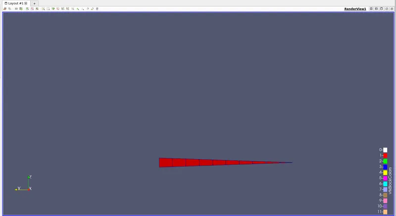
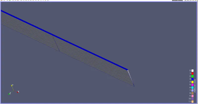
As you can see below the there is Geomtry with meshing of lenght at x axis is '0 to 2.8' at y axis '0 to 0.009994' and at z axis '-0.000349 to 0.000349'.
Angle and diameter as '4 rad and 0.002'.
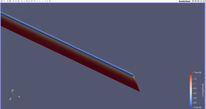
Velocity U:
This is the velocity contour of the geometry from inlet to the outlet. Where the velocity of the geometry is less nearer to the walls and more at farthest to walls.
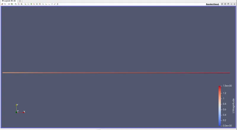
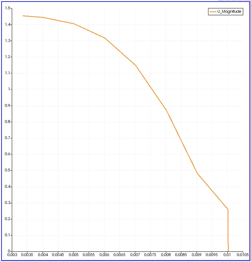
This is the velocity at the outlet of the geometry
Below is the velocity profile of the geometry from inlet to outlet.
Pressure p:
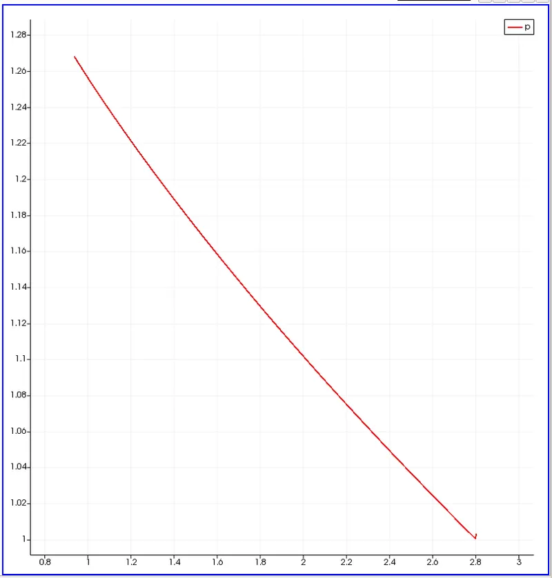
This is the pressure contour of the geometry where we can see the pressure decreases from inlet to outlet .
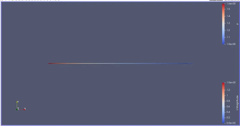
This is pressure contour of the geometry where the pressure is decresing with respect to time from inlet to outlet.
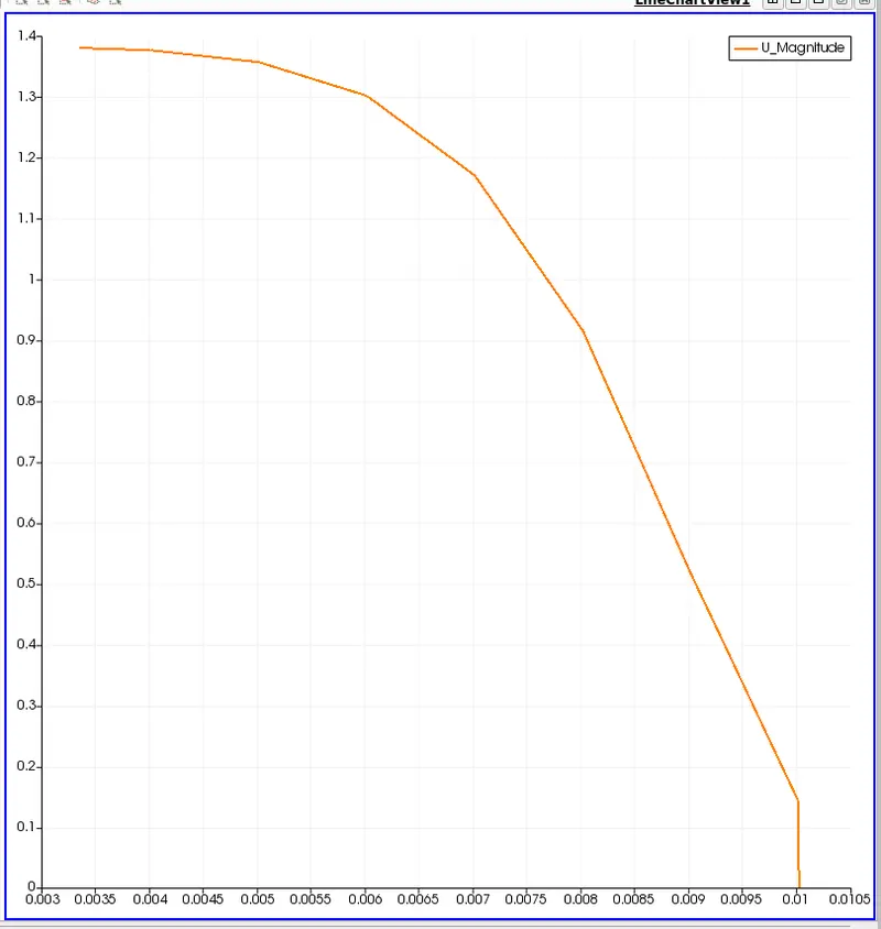
Validating the fully developed flow velocity profile with its analytical profile:
The fully developed flow is at the lenght 1.9 form the inlet of the geometry.
The analytical profile of the geometry from the matlab.
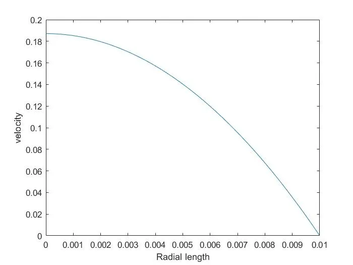
As you can see the both the profiles of velocity from the above figures.
Validating maximum velocity and pressured drop for fully developed flow:
The pressure drop at the fully developes flow at lenght 1.9 is constant as shown in the pressure profile.
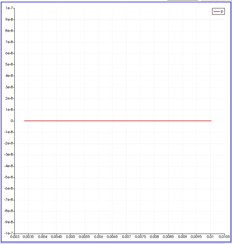
At constant pressure the velocity is maximum in the geometry.
At length 1.5 from the inlet:
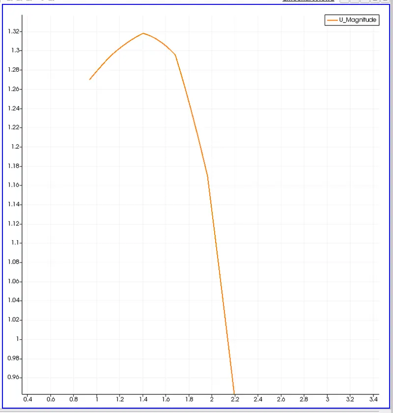
At length 1 from the inlet:
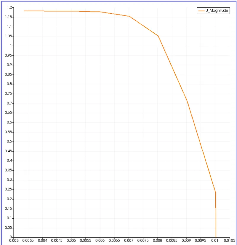
At length 2.3 from the inlet:
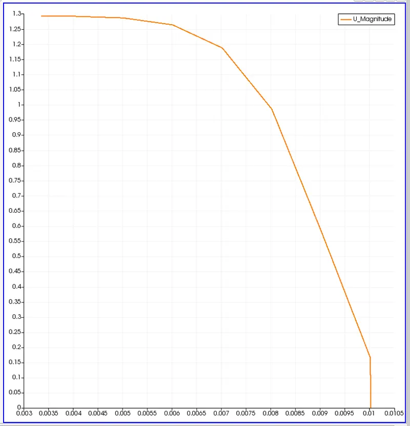
At length 2.5 from the inlet
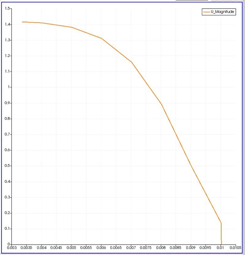
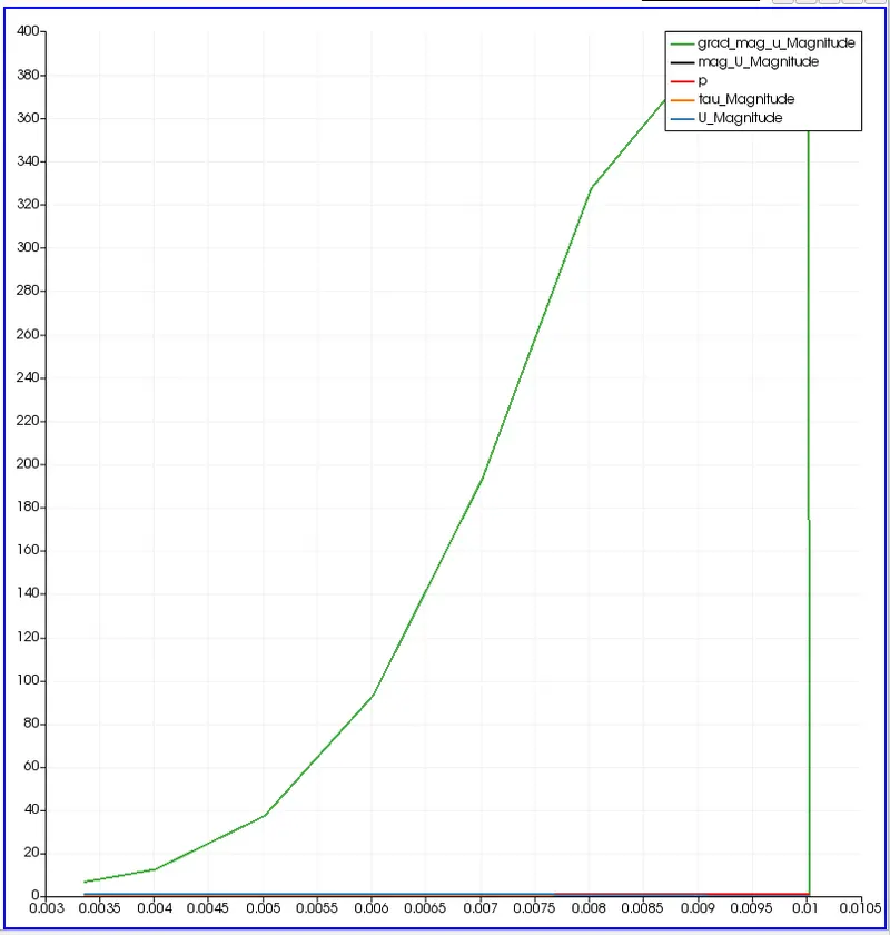
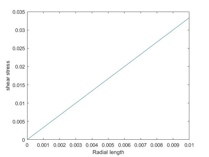
Post-process Shear stress and validate wall shear stress for fully developed flow:
Shear stress is deformation of material by slippage along a plane.
Mathematical expression: `tau=mu(du)/(dx)`
Shear stress graph of fully developed flow:
Analytical shear stress graph obtained by MATLAB:
Conclusion:
The fully developed flow velocity profile is obtained at length 1.9 from the inlet of the geometry.
The pressure is decreasing from the inlet to the outlet in the geometry.
By comparing the pressure drop and maximum velocity for fully developed flow we can say that the oulet the pressure decreses rapidly.