Challenge

Week 5.1 - Mid term project - Solving the steady and unsteady 2D heat conduction problem

RRishikesh Rao Namineni28 Aug 2022

For steady state 2D heat Conduction problem:-

Solving the Steady State 2D heat conduction equation by using the point iterative techniques. The Boundary conditions for the problem are as follows;

Top Boundary = 600 K

Bottom Boundary = 900 K

Left Boundary = 400 K

Right Boundary = 800 K

Absolute error criteria is 1e-4

Steady State 2D heat conduction equation-

The laplace Equation for the two dimension steady state with no heat transfer is:

`(partial^2T)/(partialx^2)+(partial^2T)/(partialy^2)=0`

It has elliptic nature properties.

We can discritize this equation by Central Differencing Scheme.

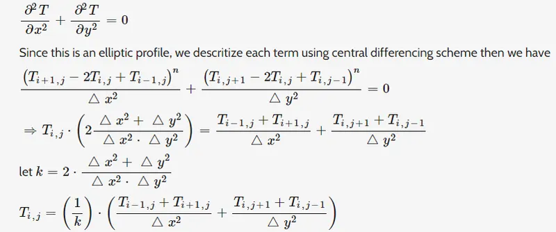
Implementing the following methods for solving implicit equations.

1. Jacobi

he Jacobi method is a method of solving a matrix equation on a matrix that has no zeros along its main diagonal (Bronshtein and Semendyayev 1997, p. 892). Each diagonal element is solved for, and an approximate value plugged in. The process is then iterated until it converges. This algorithm is a stripped-down version of the Jacobi transformation method of matrix diagonalization.

The Jacobi method is easily derived by examining each of the equations in the linear system of equations in isolation. If, in the th equation

solve for the value of while assuming the other entries of remain fixed. This gives

which is the Jacobi method.

In this method, the order in which the equations are examined is irrelevant, since the Jacobi method treats them independently. The definition of the Jacobi method can be expressed with matrices as

where the matrices D, -L, and -U represent thediagonal, strictly lower triangular, and strictly upper triangular parts of A, respectively.

now what happens when represent them as jacobi

2. Gauss-seidel

Iterative methods Jacobi and Gauss-Seidel in numerical analysis are based on the idea of successive approximations. This iterative method begins with one or two initial approximations of the roots, with a sequence of approximations x₁, x₂, x₃, …, x_k, …, as k → ∞, this sequence of roots converges to exact root 𝛼. For a system of equations Ax = B, we begin with an initial approximation of solution vector x = x_o, by which we get a sequence of solution vector x₁, x₂, …, x_k, … as k → ∞, this sequence converges to the solution x = A^{– 1}B.

The general iterative formulas can be given as:

x_{k + 1}= Hx_k ; k = 1, 2, 3, …

Where x_{k + 1} and x_k are approximations for the exact root of Ax = B at (k + 1)th and kth iterations. H is an iteration matrix that depends on A and B.

Convergence of Iterative Methods: The sequence of iterates {x_k} is said to be converging to the exact root x, if

`lim x_k=x or |xf−x|≤ε`

Where 𝜀 is a very small positive quantity called error tolerance or error bound.

for Gauss seidel as per steady state equation

3. Successive over-relaxation

The successive overrelaxation method (SOR) is a method of solving a linear system of equations derived by extrapolating the Gauss-Seidel method. This extrapolation takes the form of a weighted average between the previous iterate and the computed Gauss-Seidel iterate successively for each component,

where denotes a Gauss-Seidel iterate and is the extrapolation factor. The idea is to choose a value for that will accelerate the rate of convergence of the iterates to the solution.

In matrix terms, the SOR algorithm can be written as

where the matrices , , and represent the diagonal, strictly lower-triangular, and strictly upper-triangular parts of , respectively.

If , the SOR method simplifies to the Gauss-Seidel method. A theorem due to Kahan (1958) shows that SOR fails to converge if is outside the interval .

In general, it is not possible to compute in advance the value of that will maximize the rate of convergence of SOR. Frequently, some heuristic estimate is used, such as where is the mesh spacing of the discretization of the underlying physical domain.

SOR is enhanced gauss-seidel method for steady state equation where nth time step and n+1 time step is all same.

where omega is the relaxation factor as 1.4.

Now writing the code for the above mentioned equation in the steady state form in matlab where we took the tolerance as 1e-4, and difference in temp is 1e-2.

clear all
close all
clc

%Steady state 2D heat conduction problem
%iterative solving

%initial conditions

nx=10;
ny=10;

%value of x and y at nodes in a discretization plane

x=linspace(0,1,nx);
y=linspace(0,1,ny);
dx=x(2)-x(1);
dy=y(2)-y(1);

% given data of boundary condition
% initial temp condition

t = 300*ones(nx,ny);
t(:,1) = 400;
t(1,:) = 600;
t(:,ny) = 800;
t(nx,:) = 900;

% defining the temperature at corner points

t(1,1) = 500;
t(nx,ny) = 850;
t(1,ny) = 700;
t(nx,1) = 650;

%time step

dt = 1e-2;
told=t;
error = 9e9;
tol = 1e-4;
k = 2*(dx^2+dy^2)/(dx^2*dy^2);

%iterative method selection
method = input('Iterative method = ');

%Jacobi Iterative Method

if(method==1)
    jacobi=1;
    while(error>tol)
        for i = 2:(nx-1)
            for j = 2:(ny-1)
                t(i,j) = (((told(i-1,j)+told(i+1,j))/(dx^2))+((told(i,j+1)+told(i,j-1))/(dy^2)))/k;
            end
        end
        error = max(max(abs(t-told)));
        told = t;
        jacobi = jacobi+1;
    end
    %plotting
    contourf(t,'ShowText','on');
    colorbar;
    text1 = sprintf('number of iteration = %d', jacobi);
    title({'Steady state heat condustion profile by jacobi'; text1});

end

%GAUSS-SEIDEL ITERATIVE METHOD

if (method==2)
    gauss = 1;
    while(error>tol)
        for i = 2:(nx-1)
            for j = 2:(ny-1)
                t(i,j) = (((t(i-1,j)+told(i+1,j))/(dx^2))+((told(i,j+1)+t(i,j-1))/(dy^2)))/k;
            end
        end
        error = max(max(abs(t-told)));
        told = t;
        gauss = gauss+1;
    end
    %plotting
    contourf(t,'ShowText','on');
    colorbar;
    text1 = sprintf('number of iteration = %d', gauss);
    title({'Steady state heat condustion profile by jacobi'; text1});
end

%SUCCESSIVE OVER RELAXATION ITERATIVE METHOD

if (method==3)
    sor = 1;
    %over relaxation factor
    omega = 1.4;
    while(error>tol)
        for i = 2:(nx-1)
            for j = 2:(ny-1)
                term1 =(t(i-1,j)+told(i+1,j))/(dx^2);
                term2 =(told(i,j+1)+t(i,j-1))/(dy^2);
                t(i,j) = ((told(i,j)*(1-omega)))+(omega*(term1+term2))/k;
            end
        end
        error = max(max(abs(t-told)));
        told = t;
        sor = sor+1;
    end
    %plotting
    contourf(t,'ShowText','on');
    colorbar;
    text1 = sprintf('number of iteration = %d', sor);
    title({'Steady state heat condustion profile by jacobi'; text1});
end

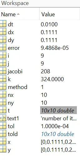
The stored value for the Jacobi Method 1 is

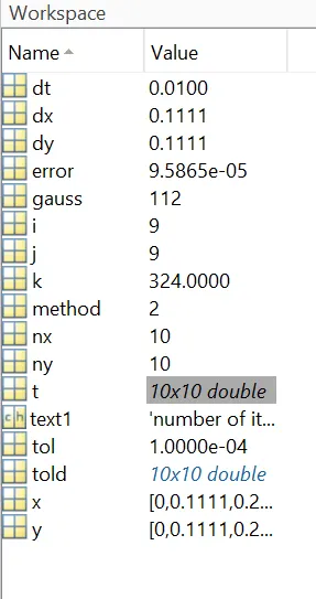
The stored value of Gauss- Siedel Method 2 is

The stored value for Successive Over Relaxation Method 3 is

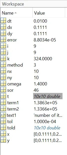
From the above figures the error values are different for all the methods and number of iterations are also different.

For Transient state 2-D heat conduction problem:-

Transient (Unsteady) state simulation:

Moving on to the Transient State simulation where we are going to work on Implicit and explicit schemes.

1. Implicit schemes

2. Explicit schemes

What is these schemes?

Explicit and implicit methods are approaches used in numerical analysis for obtaining numerical approximations to the solutions of time-dependent ordinary and PDEs, as is required in computer simulations of physical process. Explicit methods calculate the state of a system at a later time from the state of the system at the current time, while implicit methods find a solution by solving an equation involving both the current state of the system and the later one.

By derivation we have here:

Applying the first heat conduction equation in (1) to node at the time moment of , the equation can be rewritten as

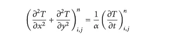
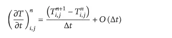
The partial differential in the two sides of (2) can be approximated by difference quotient. The temperature item in the right of the equal sign can be approximated by first-order time forward difference quotient.

The second-order partial differential in the left of the equal sign can be approximated by the central difference quotient.

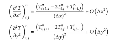
Substituting the value, we can get the difference equation of

Equation is the difference equation of heat conduction equation, and the truncation error [34] is O(DT + x2. y2).

Assuming that deltax = deltay = delta and substituting it into the latest eq., we can obtain

While we discretize the whole equation we get here.

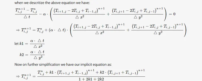
By substituting the discrtize values to Jacobi, Gauss-seidel and SOR. we get

Jacobi for Transient equation

Gauss Siedel for transient equation

Successive over Relaxation for transient equation

Writing down the code for the Transient Floe 2D heat conduction equations.

% Solving Transient flow 2D heat conduction problem
% Transient state solution with IMPLICIT
% Iterative solver - Jacobi, Gauss -seidel, Relaxation methods


clear all
close all
clc

%initial conditions
nx = 10;
ny = 10;

% No.of steps
nt = 300;

%value of x and y at nodes in a discretization plane
x = linspace(0,1,nx);
y = linspace(0,1,ny);
dx = x(2) - x(1);
dy = y(2) - y(1);


% given data of boundary condition
% initial temp condition

t = 300*ones(nx,ny);
t(:,1) = 400;
t(1,:) = 600;
t(:,ny) = 800;
t(nx,:) = 900;

% defining the temperature at corner points

t(1,1) = 500;
t(nx,ny) = 850;
t(1,ny) = 700;
t(nx,1) = 650;

%time step
dt = 0.01;
told=t;

% Thermal diffusivity
alpha = 0.3;
tprev_dt = told;

tol = 1e-4;
k1 = alpha*dt/(dx^2);
k2 = alpha*dt/(dy^2);

%iterative method selection
method = input('Iterative method = ');

%JACOBI ITERATIVE METHOD

if (method==1)
    jacobi = 1;
    for p = 1:nt
        error =99;
        while(error>tol)
            for i = 2:(nx-1)
                for j = 2:(ny-1)
                    term1 = (1+(2*k1)+(2*k2))^-1;
                    term2 = k1*term1;
                    term3 = k2*term1;
                    h = (told(i-1,j)+told(i+1,j));
                    v = (told(i,j+1)+told(i,j-1));
                    t(i,j) = ((tprev_dt(i,j)*term1)+(h*term2)+(v*term3));
                end
            end

            error = max(max(abs(t-told)));
            told = t;
            jacobi = jacobi+1;
        end
        tprev_dt = t ;
    end

    %plotting
    contourf(x,y,t,'ShowText','on');
    colorbar;
    colormap(jet);
    text1 = sprintf('number of iteration = %d', jacobi);
    title({'Transient state heat conduction profile Implicit-Jacobi'; text1});
end

%GAUSS-SEIDEL ITERATIVE METHOD

if (method==2)
    gauss = 1;
    for p = 1:nt
        error =99;
        while(error>tol)
            for i = 2:(nx-1)
                for j = 2:(ny-1)
                    term1 = (1+(2*k1)+(2*k2))^-1;
                    term2 = k1*term1;
                    term3 = k2*term1;
                    h = (t(i-1,j)+told(i+1,j));
                    v = (told(i,j+1)+t(i,j-1));
                    t(i,j) = ((tprev_dt(i,j)*term1)+(h*term2)+(v*term3));
                end
            end
            error = max(max(abs(t-told)));
            told = t;
            gauss = gauss+1;
        end
        tprev_dt = t;
    end

    %plotting
    contourf(x,y,t,'ShowText','on');
    colormap(jet);
    colorbar;
    text1 = sprintf('number of iteration = %d', gauss);
    title({'Transient state heat conduction profile Implicit-Gauss-seidel'; text1});
end

%SUCCESSIVE OVER RELAXATION ITERATIVE METHOD

if (method==3)
    sor = 1;
    % Over relaxation factor
    omega = 1.2;
    for p = 1:nt
        error =99;
        while(error>tol)
            for i = 2:(nx-1)
                for j = 2:(ny-1)
                    term1 = (1+(2*k1)+(2*k2))^-1;
                    term2 = k1*term1;
                    term3 = k2*term1;
                    h = (t(i-1,j)+told(i+1,j));
                    v = (told(i,j+1)+t(i,j-1));
                    t(i,j) = (told(i,j)*(1-omega))+(omega*((tprev_dt(i,j)*term1)+(h*term2)+(v*term3)));
                end
            end
            error = max(max(abs(t-told)));
            told = t;
            sor = sor+1;
        end
        tprev_dt = t ;
    end
    %plotting
    contourf(x,y,t,'ShowText','on');
    colormap(jet);
    colorbar;
    text1 = sprintf('number of iteration = %d', sor);
    title({'Transient state heat conduction profile Implicit-SOR'; text1});
end

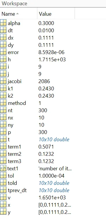
The stored value for the Jacobi Method 1 is

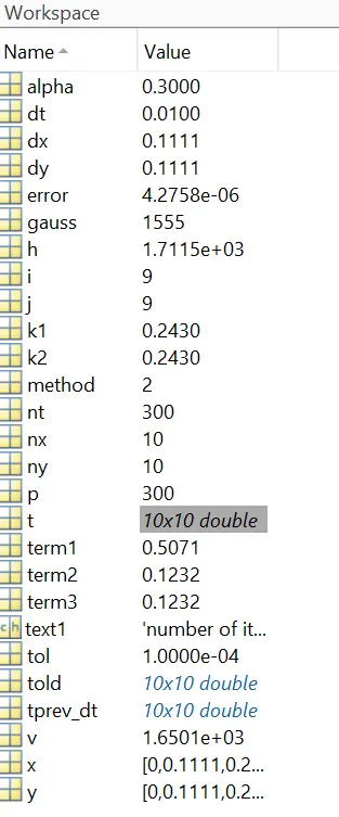
The stored value of Gauss- Siedel Method 2 is

The stored value for Successive Over Relaxation Method 3 is

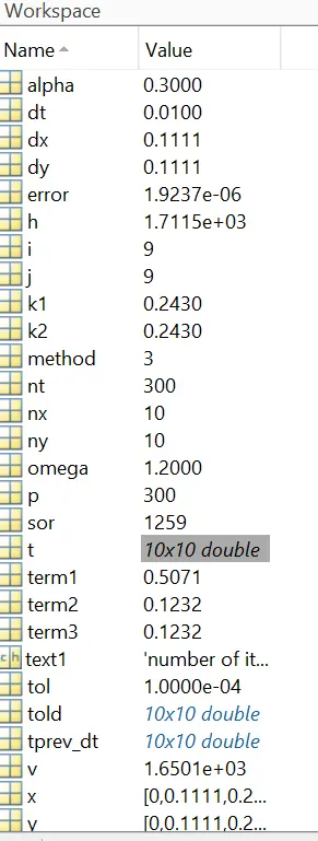
From the above figures the error values are different for all the methods and number of iterations are also different.

The final equations we end up before developing it into a computer program are as follows:

For Explicit method,

Program for explicit.

%EXPLICIT METHOD:

clear all
close all
clc

L=1;
nx=input('For the uniformly space grid please enter the number of grid points:');
ny=nx;
x=linspace(0,L,nx);
y=linspace(L,0,ny);
dx=L/(nx-1);
dy=L/(ny-1);
dt=0.001;
error=9e9;
tol=1e-4;
T_L=400;
T_R=800;
T_T=600;
T_B=900;
T=300*ones(nx,ny);
T(1,:)=T_B;
T(end,:)=T_T;
T(:,1)=T_L;
T(:,end)=T_R;
T(1,1)=(900+400)/2;
T(1,end)=(900+800)/2;
T(end,1)=(400+600)/2;
T(end,end)=(800+600)/2;
alpha=1.4;
k1=alpha*dt/dx^2;
k2=alpha*dt/dy^2;
[X,Y]=meshgrid(x,y);
Told=T;
CFL=k1+k2;
unsteady_explicit_iter=1;

for nt=1:1400
    while(error>tol)
        for i=2:nx-1
            for j=2:ny-1
                term1=Told(i-1,j)-2*Told(i,j)+Told(i+1,j);
                term2=Told(i,j-1)-2*Told(i,j)+Told(i,j+1);
                T(i,j)=Told(i,j)+k1*term1+k2*term2;
            end
        end
        error=max(max(abs(Told-T)));
        Told=T;
        unsteady_explicit_iter=unsteady_explicit_iter+1;
        contourf(T,'ShowText','on');
        colorbar;
        colormap(jet);
        text=sprintf('Unsteady Explicit Iterations = %d',unsteady_explicit_iter);
        title(text);
    end
end

The stored value for the explicit scheme is

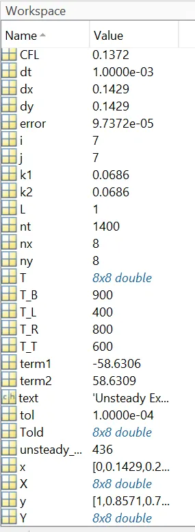
As we can see for the each and every method the error and the iterated values are different.

Week 5.1 - Mid term project - Solving the steady and unsteady 2D heat conduction problem

Ship work like this
in your own course.

Talk to a career counsellor

Ship work like thisin your own course.

Talk to a career counsellor

Ship work like this
in your own course.