Week 4.1 - Solving second order ODEs

A program that solves the following ODE. This ODE represents the equation of motion of a simple pendulum with damping

In the above equation,

g = gravity in m/s2,

L = length of the pendulum in m,

m = mass of the ball in kg,

b=damping coefficient.

Writing a program in Matlab that will simulate the pendulum motion.

use,

L=1 metre,

m=1 kg,

b=0.05.

g=9.81 m/s2.

Simulate the motion between 0-20 sec, for angular displacement=0, angular velocity=3 rad/sec at time t=0.

Below is the Program code to write in Matlab for the simulation of the pendulum as mentioned above.

The objective of the program is:

This program defines the parameters L, m, b, and g as given in the problem statement. The initial conditions for angular displacement and angular velocity are also defined as theta0 and omega0, respectively. The time span for the simulation is set to [0, 20] seconds.

The program then defines an anonymous function f that represents the second-order ODE for the motion of a simple pendulum with damping. This function takes as input the time t and a vector y containing the angular displacement and angular velocity, and returns a vector containing the first derivative of these two quantities.

The ODE is then solved using the ode45 function, which is a built-in solver for non-stiff ODEs in MATLAB/Octave. The results are stored in the vectors t and y, where t contains the time points at which the solution was evaluated, and y contains the corresponding values of angular displacement and angular velocity.

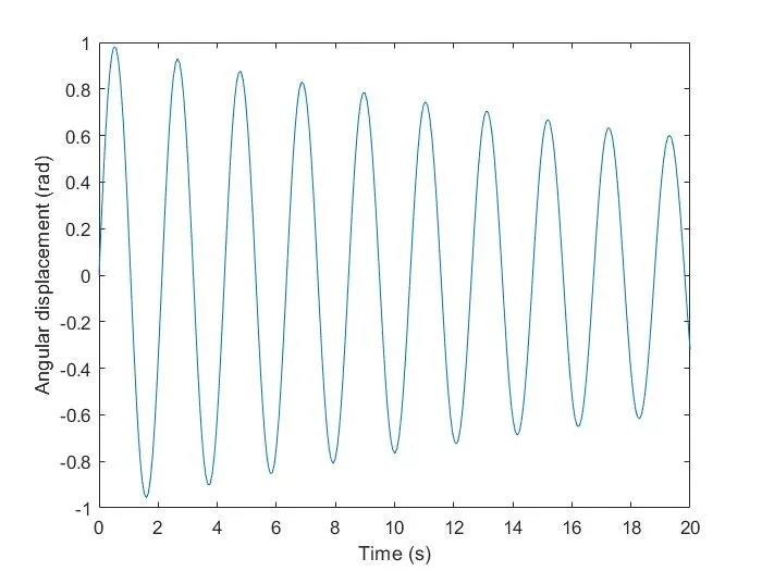
Finally, the program plots the angular displacement as a function of time using the plot function. The resulting plot shows how the angular displacement of the pendulum changes over time.

clear all
close all
clc

L = 1; % Length of pendulum (m)
m = 1; % Mass of ball (kg)
b = 0.05; % Damping coefficient
g = 9.81; % Gravity (m/s^2)

% Initial conditions
theta0 = 0; % Initial angular displacement (rad)
omega0 = 3; % Initial angular velocity (rad/s)

% Time span
tspan = [0, 20];

% Solve ODE
[t, y] = ode45(@(t, y) [y(2); -b/m*y(2) - g/L*sin(y(1))], tspan, [theta0, omega0]);

% Plot results
figure;
plot(t, y(:,1));
xlabel('Time (s)');
ylabel('Angular displacement (rad)');

% Animate pendulum motion   
figure;
for i = 1:length(t)
    x = L*sin(y(i,1));
    ycoord = -L*cos(y(i,1));
    plot([-1, 1], [0, 0], 'k', 'LineWidth', 2);
    hold on;
    plot([0, x], [0, ycoord], 'k', 'LineWidth', 2);
    plot(x, ycoord, 'ro', 'MarkerSize', m*10, 'MarkerFaceColor', 'r');
    axis([-1.5, 1.5, -1.5, 1.5]);
    drawnow;
    hold off;
end

Below is the attached result of the program with the plot and animation video.