Week 4 - CHT Analysis on Exhaust port

ABSTRACT:

To Give a brief description of why and where a CHT analysis is used while Maintaining the y+ value according to the turbulence model and justify the results. To Calculate the wall/surface heat transfer coefficient on the internal solid surface & show the velocity & temperature contours in appropriate areas. How would we verify if the HTC predictions from the simulations are right? On what factors does the accuracy of the prediction depend on? Based upon the requirements we have to analyse the HTC in 2 cases.

HEAT TRANSFER CONJUGATE:

Conjugate heat transfer is a type of heat transfer analysis between solids and fluid(s). This type of heat transfer includes both convection (between fluids) and conductive (between solids) heat transfer, as well as both forced and natural convection. Common applications and use cases of this thermal simulation type include electronics cooling, heat exchangers, industrial machinery, some AEC cases, and more.[1]

Thermal analysis is an analytical technique whereby changes in the physical state of a substance or its products are evaluated as a function of temperature and time (in some cases). The type of physical change being studied determines the choice of analysis technique, one of which is computational fluid dynamics (CFD) thermal analysis. CFD thermal analysis couples the effects of heat transfer—i.e., conduction, convection, and radiation—with fluid physics to provide realistic solutions.[2]

Thermal analysis can be steady-state or transient. The result from a steady-state thermal analysis is often used as a precursor for transient analysis, such as where the results from the former are used as initial conditions for the latter. Steady-state thermal analysis is used for determining temperatures, heat fluxes, and heat flow rates, while transient thermal analysis determines time-dependent thermal quantities.

Heat transfer has broad application to the functioning of numerous devices and systems. Heat-transfer principles may be used to preserve, increase, or decrease temperature in a wide variety of circumstances.

Y+:

The wall functions rely on the universal law ofthe wall, which basically states that the velocity distribution very near to a wall is similar for almost all turbulent flows. One of the most prominent parameters when judging the applicability of wall functions is the so-called dimensionless wall distance y+ denoted by:

`y^+=(y u_t)/(nu)`

y= Absolute distace from wall to the cell

`u_t`= friction Velocity

`nu`= Kinematic viscosity

Yplus is a dimensionless unit.

Exhaust Port:

Exhaust ports are typically used on garage doors to allow the fumes from automobiles to leave the garage, protecting the people inside. Exhaust ports are made in three thicknesses: 1/4", 2" and 3". They are made to allow for four outside diameters of exhaust hoses: 3", 4", 5" and 6". You should note that exhaust hoses tend to be measured by their inside diameter.[3]

Geometry of the exhaust port:

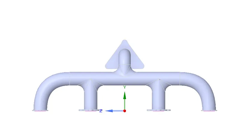
The geometry of the exhaust port which is shown below, is to determine the inlet and outlet of the fluid where there are 4 inlet and 1 outlet. The first geometry shows the outer wall of he exhaust port.

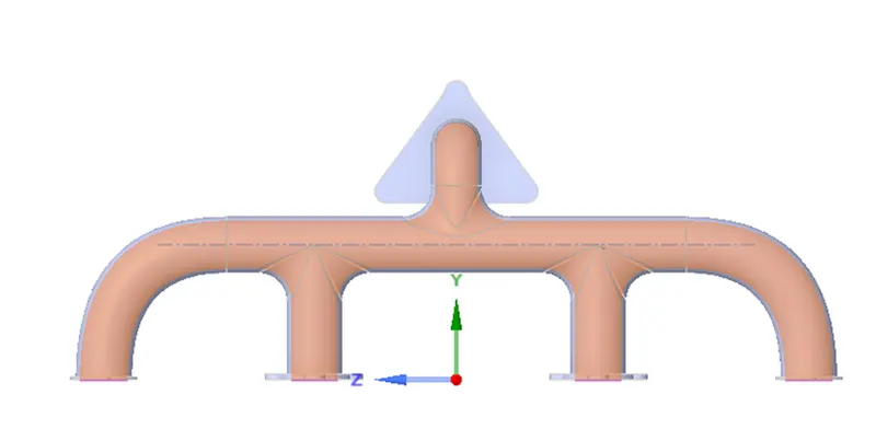
The second geometry shows the inner wall of the exhaust port which have been extruded from the geometry. From the inner wall only fluid flows where it get interact with the wall and there the convection takes place from fluid to solid.

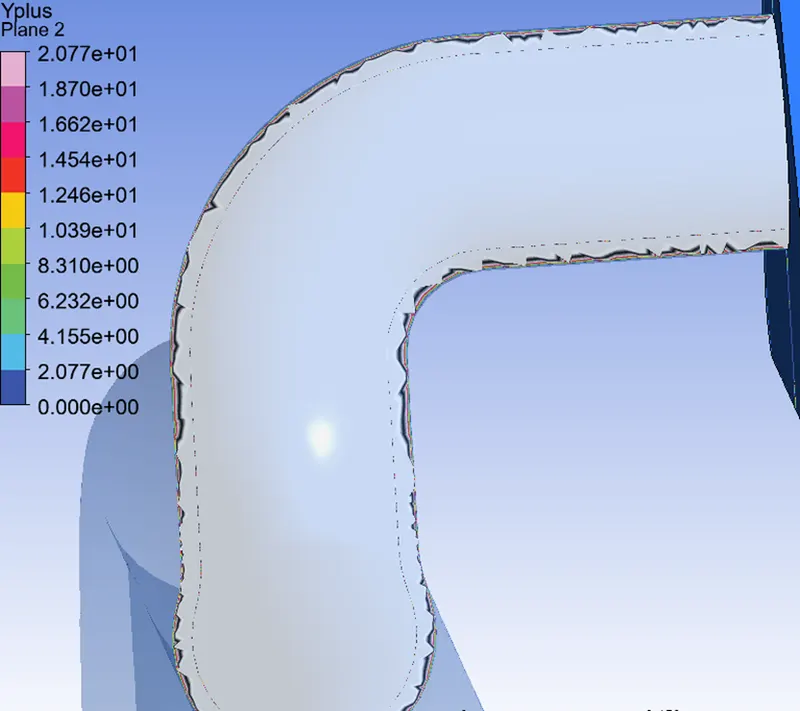
For the given data the y plus Value for the Exhaust port, according to the tuebulence keeps on changing which is being mentioned below where we can see the viscous sub layer with low velocity and then the velocity of the fluid increases gradually from the inner surface of the exhaust port.

The outlet of the exhaust port with Yplus Contour:

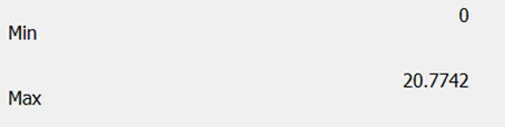
Yplus value at from min to max after the anaylysis of the geometry from the ansys:

Solving approach

• The exhaust port was modeled into the Space claim.
• The exhaust port is a three-dimensional model containing four inlets and one outlet. Despite having isothermal boundary conditions and a uniform flow rate at the four inlets, the model cannot be cut into two halves to save computational time because of its asymmetrical nature. Therefore, the whole model is discretized and is considered for meshing.
• CHT analysis requires both the solid and the liquid volume under consideration, Space claim gives an option of volume extract for selecting edges for fluid volume.
• Both the solid volume and liquid volume are copied into one component.
• Share topology is created.
• Space claim gives an option for share coincident topology, when share coincident topology is selected and executed, the mesh from the fluid volume and the solid volume are said to be conformal with each other which is a requirement for CHT analysis.
• The exhaust port is loaded into the meshing window and then simulated for baseline mesh and the refined mesh.
• The named selections are created (inlet, outlet, outer wall convection)
• The necessary contour images and graphs are studied to understand the behavior of temperature, velocity, and surface heat transfer coefficient at the interface.

Modelling Approach:

• Importing the Geometry to space claim where we can do the necessary changes for the geometry. For Example: Extruding the inner and outer walls of the geometry as mentioned above.
• In spaceclaim share the topolgy of the geometry for the confined mesh so that the mesh can be generated accurately.
• Then Generating the meshing by opening the mesh. Mesh can be generated by depending upon the requirement of the user.
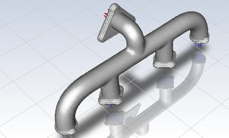
• After generating the mesh naming it with different boundary conditions for functioning of the Geometry.

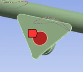
Oulet:

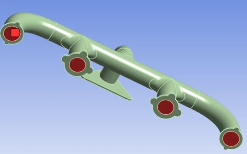
Inlet:

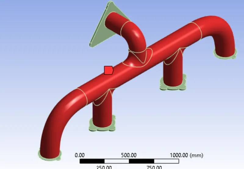
Outer Wall Convection:

• Velocity inlet will be 5m/s.
• Pressure oultlet will be 0Pa.
• Outer wall convection Heat transfer coefficient will be`20((W)/(m^2k))` free stream temperature 300K. The flanges around the inlet and the component encompassing the outlet are adiabatic (no heat transfer takes place through these walls).

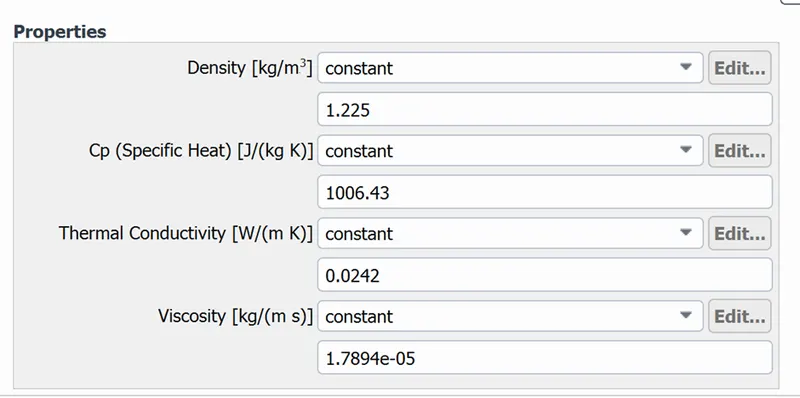
Fluid Properties inside the exhaust:

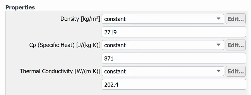
Solid Properties of the Geometry:

Case 1):

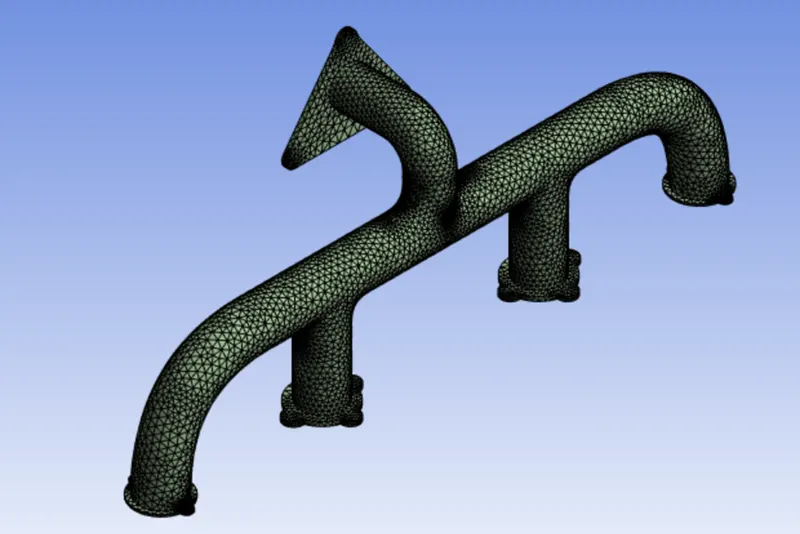
In this case, the default element size of ANSYS-FLUENT is used (150mm).

Meshing Geomtetry with no of nodes are nearly 3,74,000.

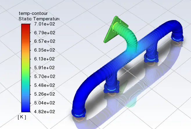
Temperature Contour:

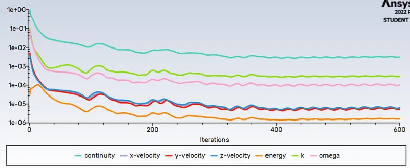
Residuals:

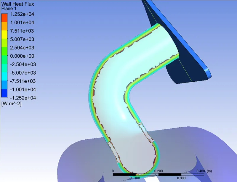
Wall Heat Flux:

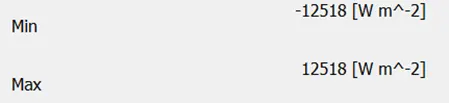
Max and min Wall Heat Flux:

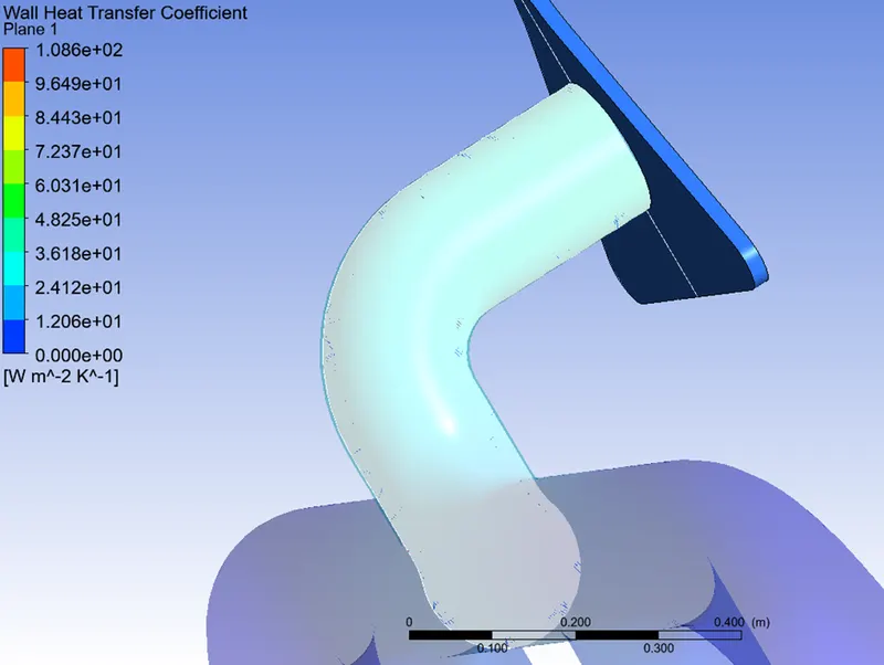
Wall Heat Transfer Coefficient :

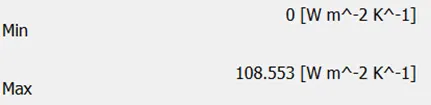
Max and Min Heat Transfer Coefficient :

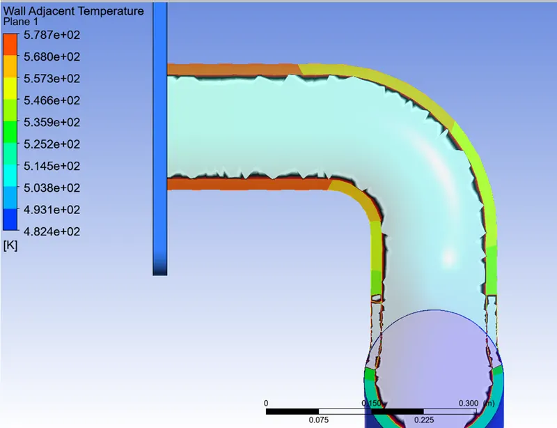
Wall Adjacent Temperature:

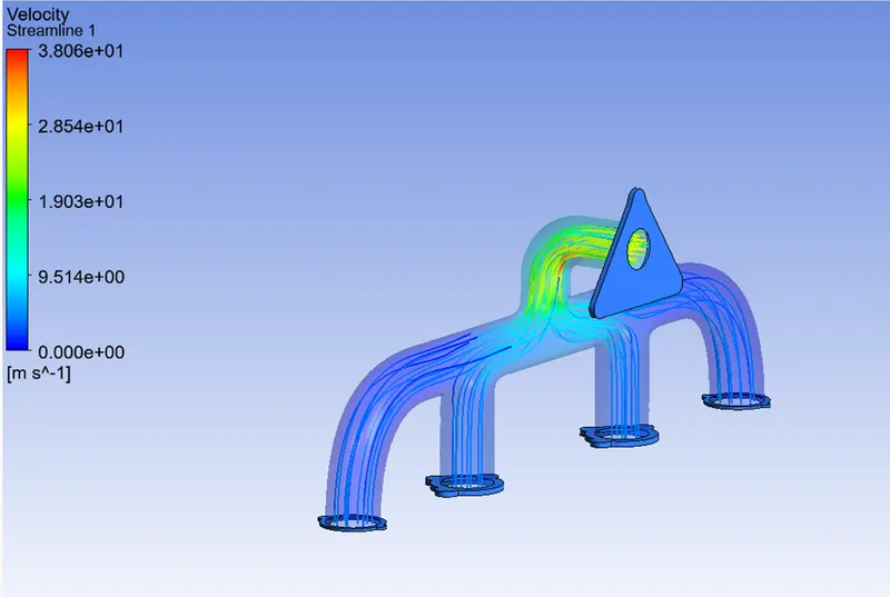
Velocity Contour With Streamline:

Case 2)

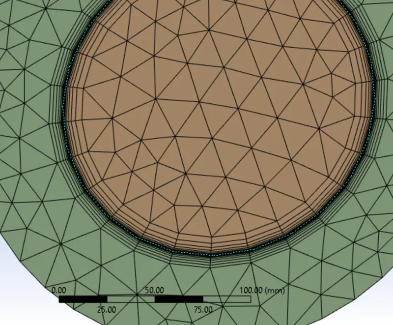
In this case, the default element size of ANSYS-FLUENT is used (20mm) with 10 inflation layers of thickness 1.5

Meshing Geomtetry with no of nodes are nearly 4,74,000.

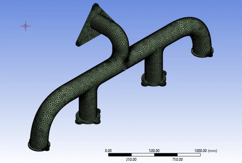
Inflation Layer Geometry with meshing:

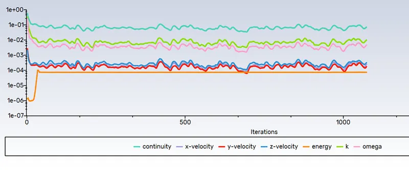
Residuals:

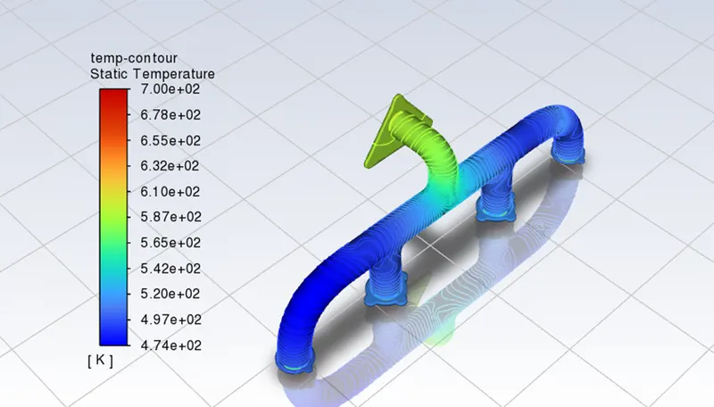
Temperature Contour:

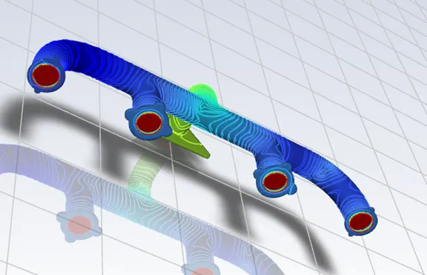
Temperature Contour for Inlet and outlet:

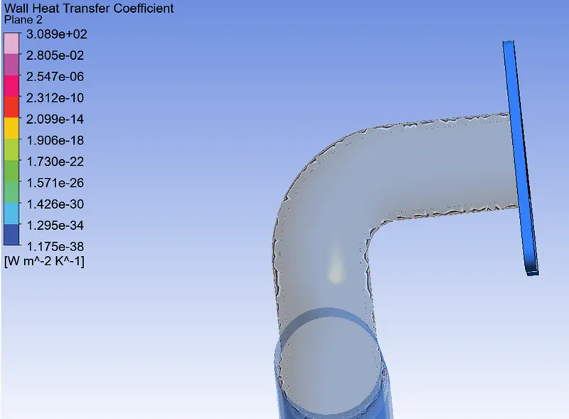
Wall Heat Transfer Coefficient:

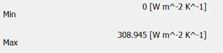
Max and Min value of Wall Heat transfer Coefficient:

In case 1 mesh generated has default setting and the results captured are less accurate due to the same.

In case 2 inflation created results in finer mesh around solid wall. Leading to a capturing temperature contour and HTC more accurately than case 1.

From above cases we notice the following results –

• Velocity tends to increase from inlet to outlet due to mass conservation and mixing of air.
• Transfer of heat from fluid to solid is high and leads to formation high velocity at the junction resulting in HTC capturing.
• The internal flow velocity and its characteristics are affected by initial velocity, pressure and physical features of geometry. Thus, CHT analysis is essential prior experimental process for better prediction product life of design component.
• As shown in the plots, the exhaust gases passing through the manifold transfers some of the heat via convection. The amount of heat transfer can be related directly with the velocity of exhaust.
• The temperature is lower where flow stagnates or is moving at the velocity. As the velocity increases, so does the Reynold’s number and the amount of heat transfer. [4]

Most accurate methods to predict results is to do a comparative study of experimental and analytical results on Nusselt’s Number. we can find the HTC theoritically with the nusselts number:

`Nu=`Convective Heat Transfer/ Condutive Heat Transfer=`h/(k/l)=(hl)/k`

h= Convective Heat Transfer Coefficint

k= Thermal Conductivity

l= Characteristic Length