Week 7 - Simulation of a 1D Super-sonic nozzle flow simulation using Macormack Method

The MacCormack method is a widely used discretization scheme for the numerical solution of hyperbolic partial differential equations.

The MacCormack method is a variation of the two-step Lax–Wendroff scheme but is much simpler in application. To illustrate the algorithm, consider the following first order hyperbolic equation:

`(partialu)/(partialt)+a(partialu)/(partialx)=0`

The application of MacCormack method to the above equation proceeds in two steps; a predictor step which is followed by a corrector step

Predictor step: In the predictor step, a "provisional" value of`u`at time level `n+1`(denoted by `u_i^(n+1)` is estimated as follows

`u_i^(n+1)=u_i^n-a(Deltat)/(Deltax)(u_(i+1)^n-u_i^n)`

The above equation is obtained by replacing the spatial and temporal derivatives in the previous first order hyperbolic equation using forward differences.

Corrector step: In the corrector step, the predicted value `u_i^(n+1)`is corrected according to the equation

`u_i^(n+1)=u_i^((n+1)/2)-a(Deltat)/(2Deltax)(u_i^(n+1)-u_(i+1)^(n+1))`

The corrector step uses backward finite difference approximations for spatial derivative. The time-step used in the corrector step is `(Deltat)/2` in contrast to the `Deltat`used in the predictor step.

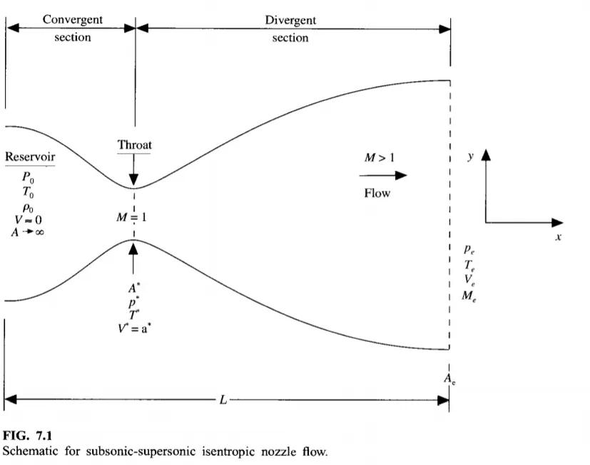
Now, We consider the study, isentropic flow through a convergent divergent nozzle. The flow at the inlet to the nozzle comes from reservoir. The cross section area of the reservoir is very large and hence velocity is very small. The flow is locally subsonic the convergent section of the nozzle, Sonic at the throat and Supersonic at the divergent section.

Considering the small control volume of the nozzle as shown in figure

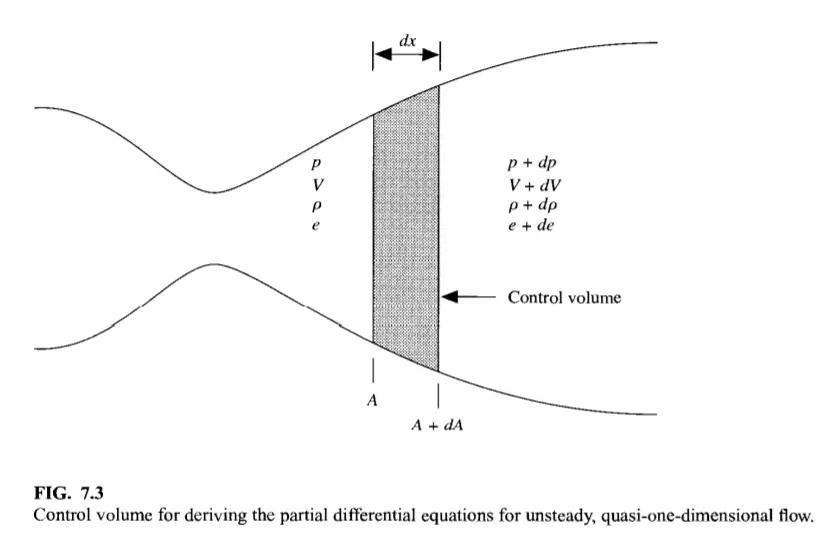
We assume that at a given section, where the cross section area is A, the flow properties are uniform across the section. Hence, although the area of the nozzle changes as a function of distance along the nozzle, X, and therefore in reality the flow field is two dimensional(the flow varies in the two dimensional x-y space), We make the assumption that the flow properties vary only with X; this is tantamount to asuming uniform flow properties across any given cross-section. Such flow is defined as Quasi one dimensional flow.

Conservative Form:

In fluid dynamics, the continuity equation states that the rate at which mass enters a system is equal to the rate at which mass leaves the system plus the accumulation of mass within the system.The differential form of the continuity equation is:

`(partialrho)/(partialt)+grad*(rhov)=0`

where

• ρ is fluid density,
• t is time,
• v is the flow velocity vector field.

The time derivative can be understood as the accumulation (or loss) of mass in the system, while the divergence term represents the difference in flow in versus flow out. In this context, this equation is also one of the Euler equations (fluid dynamics). The Navier–Stokes equations form a vector continuity equation describing the conservation of linear momentum.

If the fluid is incompressible (volumetric strain rate is zero), the mass continuity equation simplifies to a volume continuity equation:

`nabla*u=0`

which means that the divergence of the velocity field is zero everywhere. Physically, this is equivalent to saying that the local volume dilation rate is zero, hence a flow of water through a converging pipe will adjust solely by increasing its velocity as water is largely incompressible.

Conservative Continuty equation:

`(partial(rho^'A^'))/(partialt)+(partial(rho^'A^'V^'))/(partialx^')=0`

Conservative Momentum equation:

`(partial(rho^'A^'V^'))/(partialt^')+(partial(rho^'A^'(U^')^2+(1/gamma)rho^'A^'))/(partialx^')=(1/gamma)rho^'((partialA^')/(partialx^'))`

Conservative Energy equation:

`(partial[rho^'(e^'/(gamma-1))+gamma/2+(V^')^2A^1])/(partialt^')+(partial[rho^'(e^'/(gamma-1))+gamma/2+(V^')^2)V^'A^'+rho^'A^'V^']/(partialx^')=0`

For air at standard conditions, `gamma=1.4`

Now, function code for conservative part :

%%CONSERVATIVE

function [mfr_c,mfr_throat_c]=conservative(L,n,nt,cfl)

x=linspace(0,L,n);
dx=x(2)-x(1);

% initial conditions rho, a, v, T, M, mfr, p
for ii=1:length(x)
    if (x(ii)<=0.5)
        rho(ii) = 1;
        T(ii) = 1;
    elseif (x(ii)>0.5) & (x(ii)<=1.5)
        rho(ii) = 1-0.366*(x(ii)-0.5);
        T(ii)= 1-0.167*(x(ii)-0.5);
    elseif (x(ii)>1.5) & (x(ii)<=3.5)
        rho(ii) = 0.634-0.3879*(x(ii)-1.5);
        T(ii)= 0.833-0.3507*(x(ii)-1.5);
    end
end
a= 1+2.2*(x-1.5).^2;     %area
g = 1.4;                 %gamma value
% solution vectors u1, u2, u3
u1 = rho.*a;
u2 = 0.59*ones(1,n);
v=u2./u1;
u3 = u1.*((T./(g-1))+(g/2).*v.^2);

M= v./(T.^0.5);          %mach number
mfr = rho.*a.*v;         %mass flow rate
p=rho.*T;                %pressure


for z=1:31               %to find dt value
    u=(T(z))^(1/2);
    dt(z) = cfl*dx/(u + v(z));
end
dt=min(dt);

for i = 1:length(nt)
    %storing initial values
    u1_old = u1;
    u2_old = u2;
    u3_old = u3;

    for j=2:n-1
        %flux vectors
        f1 = u2;
        f2 = ((u2.^2)./u1)+((g-1)/g)*(u3-((g/2)*(u2.^2)./u1));
        f3 = ((g.*u2.*u3)./u1) - ((g*(g-1)/2)*(u2.^3)./(u1.^2));
        %source term
        j1 = (1/g)*rho(j)*T(j)*((a(j+1)-a(j))/dx);
        %predictor step
        du1_dt_p(j)= -(f1(j+1)-f1(j))/dx;           %continuity
        du2_dt_p(j)= -(f2(j+1)-f2(j))/dx + j1;      %momentum
        du3_dt_p(j)= -(f3(j+1)-f3(j))/dx;           %energy
        %updating solution vectors
        u1(j) = u1_old(j) + du1_dt_p(j)*dt;
        u2(j) = u2_old(j) + du2_dt_p(j)*dt;
        u3(j) = u3_old(j) + du3_dt_p(j)*dt;
        %updating primitives
        rho=u1./a;
        T=(g-1).*(u3./u1-(g/2).*(u2./u1).^2);
        %updating flux terms
        f1=u2;
        f2=u2.^2./u1+((g-1)/g).*(u3-(g/2)*u2.^2./u1);
        f3=g.*u2.*u3./u1-0.5*g*(g-1).*u2.^3./u1.^2;
        %source term for corrector step
        j2 = (1/g)*(rho(j)*T(j)*(a(j)-a(j-1))/dx);
        %corrector step
        du1_dt_c(j) = -(f1(j)-f1(j-1))/dx;            %continuity
        du2_dt_c(j) = -(f2(j)-f2(j-1))/dx + j2;       %momentum
        du3_dt_c(j) = -(f3(j)-f3(j-1))/dx;            %energy
    end
    %average time derivatives
    du1_dt_avg = 0.5*(du1_dt_p + du1_dt_c);
    du2_dt_avg = 0.5*(du2_dt_p + du2_dt_c);
    du3_dt_avg = 0.5*(du3_dt_p + du3_dt_c);
    %final corected values
    for k = 2:n-1
        u1(k) = u1_old(k) + du1_dt_avg(k)*dt;
        u2(k) = u2_old(k) + du2_dt_avg(k)*dt;
        u3(k) = u3_old(k) + du3_dt_avg(k)*dt;
    end
    %entry boundary conditions
    u1(1) = a(1);
    u2(1) = 2*u2(2)-u2(3);
    u3(1) = u1(1)*(T(1)/(g-1) + (g*(u2(1)/u1(1))^2)/2);
    %exit boundary conditions
    u1(n) = 2*u1(n-1)-u1(n-2);
    u2(n) = 2*u2(n-1)-u2(n-2);
    u3(n) = 2*u3(n-1)-u3(n-2);

    %Final update of primitives
    rho = u1./a;
    v = u2./u1;
    T=(g-1).*(u3./u1-(g/2).*(u2./u1).^2);
    p = rho.*T;
    M= v./T.^0.5;
    error(k) =  abs(v(k)-v(k-1));
    mfr= u2;
    %to find values at throat point
    T_throat(i) = T(16);
    rho_throat(i) = rho(16);
    v_throat(i) = v(16);
    M_throat(i) = M(16);
    p_throat(i) = p(16);
    error_throat(i)=error(16);
    mfr_throat(i)=mfr(16);

    if n==31
        for ii=[1:50:201 700]
            if ii==i
                figure(4);
                plot(x,mfr,'linewidth',1);
                hold on
                title ('Conservative form');
                xlabel('Length of nozzle');
                ylabel('Mass flow rate');
            elseif i==1400
                plot(x,mfr,'*r');
                legend('@1','@51','@101','@151','@201','@700','@1400');
            end
        end
    end

end
if n==31
    figure(5)
    plot(x,v,'b',x,p,'r',x,T,'k',x,rho,'m',x,M,'g',x,mfr,'c');
    ylim([-0.1 3.7])
    title (sprintf('Time step = %d',i));
    xlabel('Length of nozzle');
    ylabel('Non dimensional parameters');
    legend('Velocity','Pressure','Temperature','Density','Mach number','Mass flow rate','location','northwest');
    title('Conservative form');

    figure (6)
    plot(nt,rho_throat) ;
    hold on
    plot(nt,v_throat,'linewidth',1);
    plot(nt,p_throat,'linewidth',1);
    plot(nt,T_throat,'linewidth',1);
    plot(nt,M_throat,'linewidth',1);
    plot(nt,mfr_throat,'linewidth',1);
    xlabel('Time steps (nt)');
    ylabel('Non dimensional parameters');
    legend('Density','Velocity','Pressure','Temperature','Mach number','Mass flow rate');
    title('Conservative form - Time-wise variation of the primitive variables at throat point i=16');
end
mfr_c=mfr;
mfr_throat_c=mfr_throat;

end

Non-Conservative Form:

The reason they are conservative or non-conservative has to do with the splitting of the derivatives. Consider the conservative derivative:

`rho(partialu)/(partialx)`

When we discretize this, using a simple numerical derivative just to highlight the point, we get:

`rho(partialu)/(partialx)=((rhou)_i-(rhou)_(i-1))/(Deltax)`

Now, in non-conservative form, the derivative is split apart as:

`rho(partialu)/(partialx)+u(partialrho)/(partialx)`

Using the same numerical approximation, we get:

%% NON CONSERVATIVE

function [mfr_nc,mfr_throat_nc]=non_conservative(L,n,nt,cfl)

x=linspace(0,L,n);
dx=x(2)-x(1);

% initial conditions rho, a, v, T, mfr, M, p
rho = 1-0.3146*x;
T= 1-0.2314*x;
v=(0.1+1.09*x).*T.^0.5;
a= 1+2.2*(x-1.5).^2;
M= v./(T.^0.5);
mfr = rho.*a.*v;
p=rho.*T;

g = 1.4;

for z=1:31
    u=(T(z))^(1/2);
    dt(z) = cfl*dx/(u + v(z));
end
dt=min(dt);

for i = 1:length(nt)
    %storing initial values
    rho_old = rho;
    T_old = T;
    v_old = v;
    for j=2:n-1
        %predictor step
        drho_dx = (rho(j+1)-rho(j))/dx;
        dv_dx = (v(j+1)-v(j))/dx;
        dT_dx = (T(j+1)-T(j))/dx;
        da_dx = (log(a(j+1))-log(a(j)))/dx;
        drho_dt_p(j) = -rho(j)*dv_dx - rho(j)*v(j)*da_dx - v(j)*drho_dx;        %continuty
        dv_dt_p(j) = -v(j)*dv_dx - (1/g)*(dT_dx + (T(j)/rho(j))*drho_dx);       %momentum
        dT_dt_p(j) = -v(j)*dT_dx - (g-1)*T(j)*(dv_dx + v(j)*da_dx);             %energy
        %updating primitives
        v(j) = v_old(j) + dv_dt_p(j)*dt;
        rho(j) = rho_old(j) + drho_dt_p(j)*dt;
        T(j) = T_old(j) + dT_dt_p(j)*dt;
        %corrector step
        drho_dx = (rho(j)-rho(j-1))/dx;
        dv_dx = (v(j)-v(j-1))/dx;
        dT_dx = (T(j)-T(j-1))/dx;
        da_dx = (log(a(j))-log(a(j-1)))/dx;
        drho_dt_c(j) = -rho(j)*dv_dx - rho(j)*v(j)*da_dx - v(j)*drho_dx;        %continuity
        dv_dt_c(j) = -v(j)*dv_dx - (1/g)*(dT_dx + (T(j)/rho(j))*drho_dx);       %momentum
        dT_dt_c(j) = -v(j)*dT_dx - (g-1)*T(j)*(dv_dx + v(j)*da_dx);             %energy
    end
    %average time derivatives
    drho_dt_avg = 0.5*(drho_dt_p + drho_dt_c);
    dv_dt_avg = 0.5*(dv_dt_p + dv_dt_c);
    dT_dt_avg = 0.5*(dT_dt_p + dT_dt_c);
    %final corected values
    for k = 2:n-1
        rho(k) = rho_old(k) + drho_dt_avg(k)*dt;
        v(k) = v_old(k) + dv_dt_avg(k)*dt;
        T(k) = T_old(k) + dT_dt_avg(k)*dt;
    end
    %entry boundary conditions
    v(1) = 2*v(2)-v(3);
    %exit boundary conditions
    v(n) = 2*v(n-1)-v(n-2);
    rho(n) = 2*rho(n-1)-rho(n-2);
    T(n) = 2*T(n-1)-T(n-2);
    %Final update of primitives
    p = rho.*T;
    M= v./T.^0.5;
    error(k) =  abs(v(k)-v(k-1));
    mfr= rho.*a.*v;
    %to find values at throat point
    T_throat(i) = T(16);
    rho_throat(i) = rho(16);
    v_throat(i) = v(16);
    M_throat(i) = M(16);
    p_throat(i) = p(16);
    error_throat(i)=error(16);
    mfr_throat(i)=mfr(16);
    if n==31
        for ii=[1:50:201 700]
            if ii==i
                figure(1)
                plot(x,mfr,'linewidth',1);
                hold on
                title ('Non-Conservative form');
                xlabel('Length of nozzle');
                ylabel('Mass flow rate') ;
            elseif i==1400
                plot(x,mfr,'*r');
                legend('@1','@51','@101','@151','@201','@700','@1400') ;
            end
        end
    end

end
if n==31
    figure(2)
    plot(x,v,'b',x,p,'r',x,T,'k',x,rho,'m',x,M,'g',x,mfr,'c');
    ylim([-0.1 3.7]);
    title (sprintf('Time step = %d',i));
    xlabel('Length of nozzle');
    ylabel('Non dimensional parameters');
    legend('Velocity','Pressure','Temperature','Density','Mach number','Mass flow rate','location','northwest');
    title('Non-Conservative form - Steady-state distribution of primitive variables inside the nozzle');

    figure (3)
    plot(nt,rho_throat)  ;
    hold on
    plot(nt,v_throat,'linewidth',1);
    plot(nt,p_throat,'linewidth',1) ;
    plot(nt,T_throat,'linewidth',1)  ;
    plot(nt,M_throat,'linewidth',1);
    plot(nt,mfr_throat,'linewidth',1);
    xlabel('Time steps (nt)');
    ylabel('Non dimensional parameters');
    legend('Density','Velocity','Pressure','Temperature','Mach number','Mass flow rate');
    title('Non-Conservative form - Time-wise variation of the primitive variables at throat point i=16');
end
mfr_nc=mfr;
mfr_throat_nc=mfr_throat;
end

close all
clear all
clc

L=3;                    %length of nozzle
n=[31 65 87];           %number of grid points
nt=1:1400;              %number of time steps
cfl = 0.5;              %CFL number
for i = 1:length(n)
    x=linspace(0,L,n(i));
    [mfr_nc,mfr_throat_nc]=non_conservative(L,n(i),nt,cfl);
    [mfr_c,mfr_throat_c]=conservative(L,n(i),nt,cfl);
    figure(7)
    subplot(2,1,1);
    plot(nt,mfr_throat_c,'b',nt,mfr_throat_nc,'r','linewidth',1)
    xlabel('Time steps (nt)');
    ylabel('Mass flow rate');
    legend('Conservative form','Non-Conservative form');
    title('Mass flow rate using "Non-Conservative form vs Conservative form" at throat point i=16');

    subplot (2,1,2);
    plot(x,mfr_c,'b',x,mfr_nc,'r','linewidth',1);
    xlabel('Length of nozzle');
    ylabel('Mass flow rate');
    legend('Conservative form','Non-Conservative form');
    title('Mass flow rate using "Non-Conservative form vs Conservative form" in the nozzle');

    figure(8)
    subplot (2,1,1);
    plot(nt,mfr_throat_c,'linewidth',1);
    hold on
    xlabel('Time steps (nt)');
    ylabel('Mass flow rate');
    legend('@31 nodes','@65 nodes','@87 nodes');
    title('Conservative form: Grid independency test at throat point i=16');
    subplot (2,1,2);
    plot(nt,mfr_throat_nc,'linewidth',1);
    hold on
    xlabel('Time steps (nt)');
    ylabel('Mass flow rate');
    legend('@31 nodes','@65 nodes','@87 nodes');
    title('Non-Conservative form: Grid independency test at throat point i=16');
    figure(9)
    subplot (2,1,1);
    plot(x,mfr_c,'linewidth',1);
    hold on
    xlabel('Length of nozzle');
    ylabel('Mass flow rate');
    legend('@31 nodes','@65 nodes','@87 nodes');
    title('Conservative form: Grid independency test along the nozzle');
    subplot (2,1,2);
    plot(x,mfr_nc,'linewidth',1);
    hold on
    xlabel('Length of nozzle');
    ylabel('Mass flow rate');
    legend('@31 nodes','@65 nodes','@87 nodes');
    title('Non-Conservative form: Grid independency test along the nozzle');

end