Week 6 - Multivariate Newton Rhapson Solver

The equation to solve:

Boundary Condition:

• Y1 = 1
• Y2 = 0
• y3 = 0
• Alpha = 1
• Time to run = 10 mins

Procedure:

The process of solving the set of equation with respect to time. The equation has to be solved every timestep. So the newton-rahpson method is used to solve in timestep and the results if flowed through the time. Function for both euler and newton-rahpson method is prepared. Since we need such type of result the newton-raphson method is incorporated in euler. so that the solution is solved with respect to the time of 10 minutes with small dt.

Program:

import numpy as np
from numpy.linalg import inv
import matplotlib.pyplot as plt 


"""t_start = 0 
t_end = 600
n = 6000

dt = (t_end - t_start)/(n-1)

iter = 1

y1 = 1
y2 = 0
y3 = 0  """

def f1(y1_old,y1,y2,y3,dt):
	return y1_old + (-0.04*y1 + pow(10,4)*y2*y3)*dt - y1

def f2(y2_old,y1,y2,y3,dt):
	return y2_old + (0.04*y1 - pow(10,4)*y2*y3 - 3*pow(10,7)*y2*y2)*dt - y2 

def f3(y3_old,y1,y2,y3,dt):
	return y3_old + (3*pow(10,7)*y2*y2)*dt - y3 

def jacobian(y1_old,y2_old,y3_old,y1,y2,y3,dt):
	J =  np.zeros((3,3))
	h = 1e-8

	J[0,0] = (f1(y1_old,y1+h,y2,y3,dt)-f1(y1_old,y1,y2,y3,dt))/h
	J[0,1] = (f1(y2_old,y1,y2+h,y3,dt)-f1(y2_old,y1,y2,y3,dt))/h
	J[0,2] = (f1(y3_old,y1,y2,y3+h,dt)-f1(y3_old,y1,y2,y3,dt))/h

	J[1,0] = (f2(y1_old,y1+h,y2,y3,dt)-f2(y1_old,y1,y2,y3,dt))/h
	J[1,1] = (f2(y2_old,y1,y2+h,y3,dt)-f2(y2_old,y1,y2,y3,dt))/h
	J[1,2] = (f2(y3_old,y1,y2,y3+h,dt)-f2(y3_old,y1,y2,y3,dt))/h

	J[2,1] = (f3(y1_old,y1+h,y2,y3,dt)-f3(y1_old,y1,y2,y3,dt))/h
	J[2,2] = (f3(y2_old,y1,y2+h,y3,dt)-f3(y2_old,y1,y2,y3,dt))/h
	J[2,2] = (f3(y3_old,y1,y2,y3+h,dt)-f3(y3_old,y1,y2,y3,dt))/h
	return J

def newtwon_raphson(y1,y2,y3,y1_guess,y2_guess,y3_guess,dt):

	y_old = np.zeros((3,1))
	y_old[0] = y1_guess
	y_old[1] = y2_guess
	y_old[2] = y3_guess

	F = np.zeros((3,1))

	error = 9e9
	tol = 1e-4
	alpha = 1
	iter = 1

	while(error>=tol):
		J = jacobian(y_old[0],y_old[1],y_old[2],y1,y2,y3,dt)
		F[0] = f1(y_old[0],y1,y2,y3,dt)
		F[1] = f2(y_old[1],y1,y2,y3,dt)
		F[2] = f3(y_old[2],y1,y2,y3,dt)

		y_new = y_old - alpha*(np.matmul(inv(J),F))

		error = np.max(np.abs(y_new - y_old))
		y_old = y_new
		log_message = 'iteration # = {0} y1 = {1} y2 = {2} y3 = {3}'.format(iter, y_new[0],y_new[1], y_new[2])
		print(log_message)
		iter = iter+1
		y1_final = y_new[0]
		y2_final = y_new[1]
		y3_final = y_new[2]

	return[y_new[0],y_new[1], y_new[2]]

def implicit_euler(y1,y2,y3,t_start,t_end,dt):
	t = np.arange(t_start,t_end,dt)
	time = len(t)
	y_1 = np.zeros(time)
	y_2 = np.zeros(time)
	y_3 = np.zeros(time)

	y_1[0] =y1
	y_2[0] = y2 
	y_3[0] = y3 

	y1_guess = 1 
	y2_guess = 0
	y3_guess = 0

	for i in range (1,time):
		y_1[i],y_2[i],y_3[i] = newtwon_raphson(y_1[i-1],y_2[i-1],y_3[i-1],y1_guess,y2_guess,y3_guess,dt)
		y1_guess = y_1[i]
		y2_guess = y_2[i]
		y3_guess = y_3[i]

	return [t,y_1,y_2,y_3]

t,y1,y2,y3 = implicit_euler(1,0,0,0,600,0.001)

plt.plot(t,y1)
plt.plot(t,y2)
plt.plot(t,y3)
plt.xlabel('Simulation Time (sec)')
plt.ylabel('Value of Variable')
plt.legend(['y1','y2','y3'])
plt.title('Multivariate Newton Rhapson Method for dt = 0.001')
plt.grid('on')
plt.show()

Result:

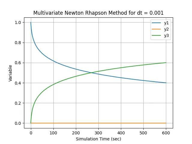
Thus The solution for the equation:

y1 = [0.39994586] y2 = [2.63125244e-06] y3 = [0.60009946]

Ideal step size selection:

The ideal step size selection i made is Trail and error with various values starting from 0.1 to 0.0001. For the values bigger than 0.001, my program end up with singularity matrix error. As the diterminant of the Jacobian matrix in the Newton-Raphson method goes zero got those valuse of dt. From dt as 0.001 and lower the program run and finds the solution. The smaller the value the more time it consumes to solve the solution. To use optimised amount of time to solve the equation properly i chose 0.001 as dt.