Week 3 - Solving second order ODEs

Equation:

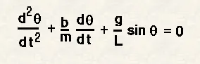
n the above equation,

g = gravity in m/s2,

L = length of the pendulum in m,

m = mass of the ball in kg,

b=damping coefficient.

Write a program in Python that will simulate the pendulum motion, just like the one shown in the start of this challenge.

use,

L=1 metre,

m=1 kg,

b=0.05.

g=9.81 m/s2.

Simulate the motion between 0-20 sec, for angular displacement=0,angular velocity=3 rad/sec at time t=0.

OdeInt:

Odeint is a modern C++ library for numerically solving Ordinary Differential Equations. It is developed in a generic way using Template Metaprogramming which leads to extraordinary high flexibility at top performance. The numerical algorithms are implemented independently of the underlying arithmetics. This results in an incredible applicability of the library, especially in non-standard environments. For example, odeint supports matrix types, arbitrary precision arithmetics and even can be easily run on CUDA GPUs - check the Highlights to learn more. Moreover, odeint provides a comfortable easy-to-use interface allowing for a quick and efficient implementation of numerical simulations. Visit the impressively clear 30 lines Lorenz example. Odeint is a header only C++ library and the full source code is available for download. distributed under the highly liberal Boost Software License. Hence, odeint is free, open source and can be used in both non-commercial and commercial applications.

Code explanation:

• With the given data the ode solver is used to solve the equation.
• As the equation is second order derivative, we need to differtiate twice the equation.
• Thus the function is used to provide the variables which is differentiate one after other.
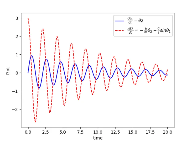
• Once the differntiation is over, the values are stored in the array is ploted and studied.
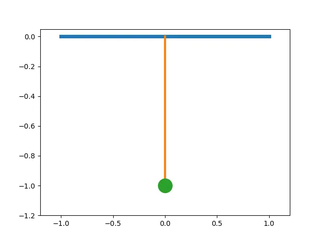
• For the pendulum motion the position of pendulum is marked with '0' and line is drawn.
• In a for loop, the plot of the pendulum position is stored and later made into animation using magick.

Program:

import math
import matplotlib.pyplot as plt
import numpy as np 
from scipy.integrate import odeint

def model(theta, t, b, g, l, m):
	theta1 =theta[0]
	theta2 = theta[1]
	dtheta1_dt = theta2
	dtheta2_dt = -(b/m)*theta2 - (g/l)*math.sin(theta1)
	dtheta_dt = [dtheta1_dt, dtheta2_dt]
	return dtheta_dt

b= 0.02
g=9.81
l=1
m=0.1

theta_0 = [0,3]

t=np.linspace(0,20,150)

theta =odeint(model, theta_0, t, args = (b,g,l,m))

X =theta[:,0]
ct = 1

plt.figure(1)
plt.plot(t,theta[:,0],'b-',label=r'$\frac{d\theta_1}{dt}=\theta2$')
plt.plot(t,theta[:,1],'r--', label=r'$\frac{d\theta2}{dt}=-\frac{b}{m}\theta_2-\frac{g}{l}sin\theta_1$')
plt.xlabel('time')
plt.ylabel('Plot')
plt.legend()
plt.show()

for Theta in X:
	x1=0
	y1=0
	
	x2 = l*math.sin(Theta)
	y2 = -(l*math.cos(Theta))
	file_name = '%03d.png'%ct
	plt.figure()
	plt.plot([-1,1],[0,0],linewidth = 5)
	plt.plot([x1,x2],[y1,y2],linewidth = 3)
	plt.plot(x2,y2,'o', markersize = 20)
	plt.xlim([-1.2,1.2])
	plt.ylim([-1.2,0.05])
	plt.savefig(file_name)
	ct = ct+1

Plot:

Animation:

Inference:

Thus a second order ODE is solved using python and results are shown.