Week 2 Air standard Cycle

Otto cycle:

An Otto cycle is an idealized thermodynamic cycle that describes the functioning of a typical spark ignition piston engine. It is the thermodynamic cycle most commonly found in automobile engines.

The Otto cycle is a description of what happens to a mass of gas as it is subjected to changes of pressure, temperature, volume, addition of heat, and removal of heat. The mass of gas that is subjected to those changes is called the system. The system, in this case, is defined to be the fluid (gas) within the cylinder. By describing the changes that take place within the system, it will also describe in inverse, the system's effect on the environment. In the case of the Otto cycle, the effect will be to produce enough net work from the system so as to propel an automobile and its occupants in the environment.

The Otto cycle is constructed from:

• Top and bottom of the loop: a pair of quasi-parallel and isentropic processes (frictionless, adiabatic reversible).
• Left and right sides of the loop: a pair of parallel isochoric processes (constant volume).

The isentropic process of compression or expansion implies that there will be no inefficiency (loss of mechanical energy), and there be no transfer of heat into or out of the system during that process. The cylinder and piston are assumed to be impermeable to heat during that time. Work is performed on the system during the lower isentropic compression process. Heat flows into the Otto cycle through the left pressurizing process and some of it flows back out through the right depressurizing process. The summation of the work added to the system plus the heat added minus the heat removed yields the net mechanical work generated by the system.

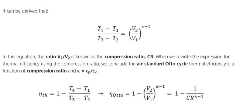
Thermal efficiency of the engine formula:

Code explanation:

• With the initial condition of the engine, the code beingines.
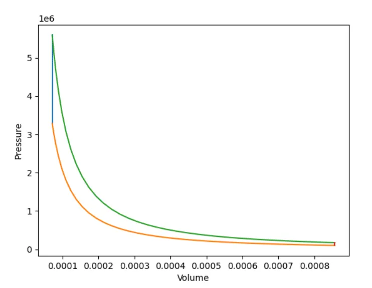
• For the PV diagram of the Otto cycle, we the need pressure and volume at each points.
• As inital conditions, We know the pressure, temperature and Engine data.
• We use ideal gas eqaution to find the next pressure and volume for next cycle.
• The cycles do have Contant volume at process of 2-3 and 4-1. Then we assume Temperature at third process because thats were the ignition occurs.
• With the values availbale and ideal equation, The pressure and volume at the end of each process is found.
• Yet, for the PV plot, we now know the points. For ploting the volume where its not constant.
• General mathematical formula is used to calculate the volume inside the engine with respect to change in crank angle in diferent function.
• The volume data is used to plot the actual PV diagram of the Otto cycle.

Program:

import math
import matplotlib.pyplot as plt

def engine_kinematics(bore, stroke, con_rod, cr, start_crank, end_crank):
	a = stroke/2
	R=con_rod/a

	v_s = (math.pi/4)*pow(bore,2)*stroke
	v_c = v_s/(cr-1)

	start_crank_angle = math.radians(start_crank)
	end_crank_angle = math.radians(end_crank)

	num_values = 50
	dtheta = (start_crank_angle - end_crank_angle)/(num_values-1)
	v =[]

	for i in range(0,num_values):
		theta =start_crank_angle+i*dtheta
		term1 = 0.5*(cr-1)
		term2 = R + 1-math.cos(theta)
		term3 = pow(R,2)-pow(math.sin(theta),2)
		term3 = pow(term3,0.5)
		v.append((1+term1*(term2-term3))*v_c)

	return v

p1 =101325
t1=500
t3=2300

gamma = 1.4

bore = 0.1
stroke =0.1
con_rod = 0.15
cr = 12

v_s = (math.pi/4)*pow(bore,2)*stroke
v_c = v_s/(cr-1)

v1 =v_c+v_s
v2 = v_c
#p2v2^gamma = p1v1^gamma
p2 = p1*pow(v1, gamma)/pow(v2,gamma)

rhs = p1*v1/t1
t2 = p2*v2/rhs

V_compression = engine_kinematics(bore, stroke, con_rod, cr, 180, 0)
constant = p1*pow(v1,gamma)
P_compression = []

for v in V_compression:
	P_compression.append(constant/pow(v,gamma))

v3=v2

rhs = p2*v2/t2
p3 = rhs*t3/v3

V_expansion = engine_kinematics(bore, stroke, con_rod, cr, 0, 180)
constant = p3*pow(v3,gamma)
P_expansion=[]

for v in V_expansion:
	P_expansion.append(constant/pow(v,gamma))

v4=v1

p4 = p3*pow(v3,gamma)/pow(v4,gamma)

t4 = p4*v4/rhs

#Efficiency Calculation
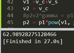
Thermal_efficiency = (1-1/pow(cr,(gamma-1)))*100
print(Thermal_efficiency)

plt.plot([v2,v3],[p2,p3])
plt.plot(V_compression,P_compression)
plt.plot(V_expansion,P_expansion)
plt.plot([v4,v1],[p4,p1])
plt.xlabel('Volume')
plt.ylabel('Pressure')
plt.show()

Plot:

Thermal efficiency result:

Inference:

Thus the otto cycle simulation is done using python program and the thermal efficiency of the cycle is found.