Week 5 - Curve fitting

Curve fitting:

Curve fitting is the process of constructing a curve, or mathematical function, that has the best fit to a series of data points, possibly subject to constraints. Curve fitting can involve either interpolation, where an exact fit to the data is required, or smoothing, in which a "smooth" function is constructed that approximately fits the data. A related topic is regression analysis, which focuses more on questions of statistical inference such as how much uncertainty is present in a curve that is fit to data observed with random errors. Fitted curves can be used as an aid for data visualization, to infer values of a function where no data are available, and to summarize the relationships among two or more variables. Extrapolation refers to the use of a fitted curve beyond the range of the observed data, and is subject to a degree of uncertainty since it may reflect the method used to construct the curve as much as it reflects the observed data.

The first degree polynomial equation

is a line with slope a. A line will connect any two points, so a first degree polynomial equation is an exact fit through any two points with distinct x coordinates.

If the order of the equation is increased to a second degree polynomial, the following results:

This will exactly fit a simple curve to three points.

If the order of the equation is increased to a third degree polynomial, the following is obtained:

Best fit:

Line of best fit refers to a line through a scatter plot of data points that best expresses the relationship between those points. Statisticians typically use the least squares method to arrive at the geometric equation for the line, either though manual calculations or regression analysis software. A straight line will result from a simple linear regression analysis of two or more independent variables. A regression involving multiple related variables can produce a curved line in some cases.

Program:

import math
import numpy as np 
import matplotlib.pyplot as plt
from scipy.optimize import curve_fit

#linear function
def linear_function(t,a,b):
	return a*t + b

#cubic function
def cubic_function(t,a,b,c,d):
	return a*pow(t,3) + b*pow(t,2) + c*t + d

def file_read():
	temperature = []
	cp = []
	for line in open('data','r'):
		values = line.split(',')
		temperature.append(float(values[0]))
		cp.append(float(values[1]))
	return[temperature,cp]

temperature, cp = file_read()
popt, pcov = curve_fit(linear_function, temperature, cp)
fit_cp_l = linear_function(np.array(temperature), *popt)
plt.figure(1)
plt.plot(temperature,cp,color = 'g')
plt.plot(temperature,fit_cp_l, color = 'b')
plt.legend(['Actual data','curve fit'])
plt.xlabel('Temperature')
plt.ylabel('cp')
plt.title('Linear curve fitting')


popt, pcov =  curve_fit(cubic_function, temperature, cp)
fit_cp_c = cubic_function(np.array(temperature), *popt)
plt.figure(2)
plt.plot(temperature,cp,color = 'g')
plt.plot(temperature,fit_cp_c, color = 'b')
plt.legend(['Actual data','curve fit'])
plt.xlabel('Temperature')
plt.ylabel('cp')
plt.title('Cubic curve fitting')
plt.show()

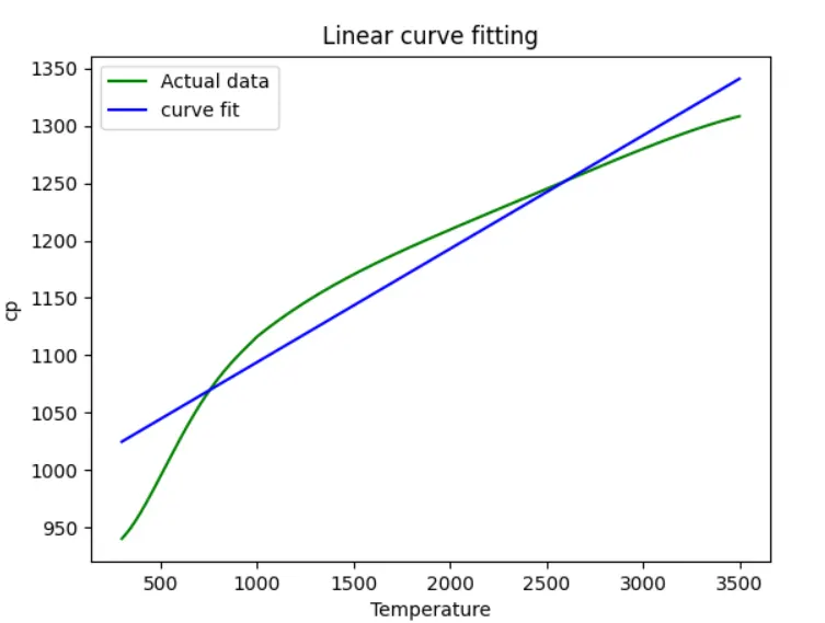
linear fit graph:

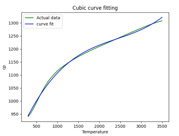
Cubic fit graph:

1. What does popt and pcov mean?

popt is a one dimensional array of the best estimates for the parameter values, each entry matches the order in the function definition. pcov is the covariance matrix showing the uncertainty and interdependence of each parameter in popt. We take the diagonal elements as pvar for the variance of each parameter in popt. The above error didn’t consider the errors in the individual data points correctly.

2. What does np.array(temperature) do?

The function of np.array(temperature) is to pass the program as well as the popt. The value of temperature through the function which is defined in the program as well as the popt. The value of temperature are saved in the data file which is copied in the same program folder.

3. What does the * in *popt mean?

The star in *popt unpacks the popt array so the two optimized parameter values become the second and third arguments to the function.

5. What needs to be done in order to make the curve fit perfect?

To make the cubic fit better, you need to split the data into smaller datasets and fit them separately.

6. Show empirically as to how well your curve has been fit.

To make a curve fit perfect the error estimates should be considered. The perfect fit is a fit where it should match the original curve and shouldn't have any scaling and centering errors in that particular degree of the polynomial. Line of best fit refers to a line through a scatter plot of data points that best expresses the relationship between those points. Statisticians typically use the least squares method to arrive at the geometric equation for the line, either though manual calculations or regression analysis software. A straight line will result from a simple linear regression analysis of two or more independent variables. A regression involving multiple related variables can produce a curved line in some cases.