Week 4.1 - Genetic Algorithm

Genetic algorithm:

In computer science and operations research, a genetic algorithm (GA) is a metaheuristic inspired by the process of natural selection that belongs to the larger class of evolutionary algorithms (EA). Genetic algorithms are commonly used to generate high-quality solutions to optimization and search problems by relying on biologically inspired operators such as mutation, crossover and selection.

At each step, the genetic algorithm uses the current population to create the children that make up the next generation. The algorithm selects a group of individuals in the current population, called parents, who contribute their genes—the entries of their vectors—to their children. The algorithm usually selects individuals that have better fitness values as parents. You can specify the function that the algorithm uses to select the parents in the SelectionFcn option. See Selection Options.

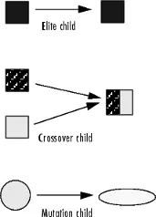
The genetic algorithm creates three types of children for the next generation:

• Eliteare the individuals in the current generation with the best fitness values. These individuals automatically survive to the next generation.
• Crossover are created by combining the vectors of a pair of parents.
• Mutation children are created by introducing random changes, or mutations, to a single parent.

The following schematic diagram illustrates the three types of children.

Mutation and Crossover explains how to specify the number of children of each type that the algorithm generates and the functions it uses to perform crossover and mutation.

The following sections explain how the algorithm creates crossover and mutation children.

Crossover Children
The algorithm creates crossover children by combining pairs of parents in the current population. At each coordinate of the child vector, the default crossover function randomly selects an entry, or gene, at the same coordinate from one of the two parents and assigns it to the child. For problems with linear constraints, the default crossover function creates the child as a random weighted average of the parents.

Mutation Children
The algorithm creates mutation children by randomly changing the genes of individual parents. By default, for unconstrained problems the algorithm adds a random vector from a Gaussian distribution to the parent. For bounded or linearly constrained problems, the child remains feasible.

The next step is to generate a second generation population of solutions from those selected through a combination of genetic operators: crossover (also called recombination), and mutation.

For each new solution to be produced, a pair of "parent" solutions is selected for breeding from the pool selected previously. By producing a "child" solution using the above methods of crossover and mutation, a new solution is created which typically shares many of the characteristics of its "parents". New parents are selected for each new child, and the process continues until a new population of solutions of appropriate size is generated. Although reproduction methods that are based on the use of two parents are more "biology inspired", some research suggests that more than two "parents" generate higher quality chromosomes.

These processes ultimately result in the next generation population of chromosomes that is different from the initial generation. Generally, the average fitness will have increased by this procedure for the population, since only the best organisms from the first generation are selected for breeding, along with a small proportion of less fit solutions. These less fit solutions ensure genetic diversity within the genetic pool of the parents and therefore ensure the genetic diversity of the subsequent generation of children.

Opinion is divided over the importance of crossover versus mutation. There are many references in Fogel (2006) that support the importance of mutation-based search.

Although crossover and mutation are known as the main genetic operators, it is possible to use other operators such as regrouping, colonization-extinction, or migration in genetic algorithms.[citation needed]

It is worth tuning parameters such as the mutation probability, crossover probability and population size to find reasonable settings for the problem class being worked on. A very small mutation rate may lead to genetic drift (which is non-ergodic in nature). A recombination rate that is too high may lead to premature convergence of the genetic algorithm. A mutation rate that is too high may lead to loss of good solutions, unless elitist selection is employed. An adequate population size ensures sufficient genetic diversity for the problem at hand, but can lead to a waste of computational resources if set to a value larger than required.

Genetic Algorithm syntax:

[x,fval] = ga(ObjectiveFunction,nvars,[],[],[],[],LB,UB, ...
    ConstraintFunction)

Program:

clear all
close all
clc

x=linspace(0,0.6,150);
y=linspace(0,0.6,150);

[xx yy]=meshgrid(x,y);
num_case=150;

for i=1:length(xx)
    for j=1:length(yy)
        input_vector(1)=xx(i,j);
        input_vector(2)=yy(i,j);
        f(i,j) = stagalmite(input_vector);
    end
end

%study1
tic 
for i=1:num_case
    [inputs,Fopt(i)]=ga(@stagalmite,2);
    xopt(i)=inputs(1);
    yopt(i)=inputs(2);
end

Study1=toc

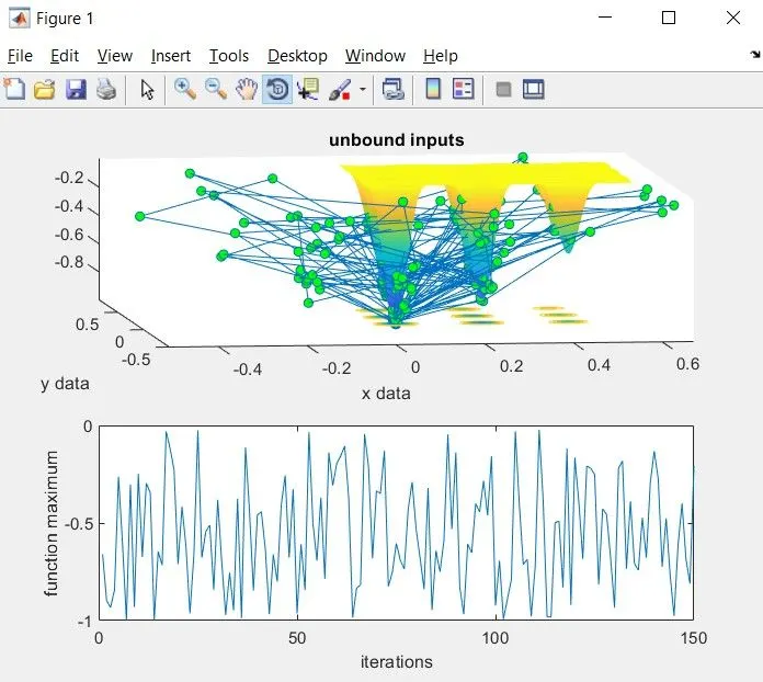
figure(1)
subplot(2,1,1);
hold on
surfc(xx,yy,f);
shading interp;
xlabel('x data');
ylabel('y data');
plot3(xopt,yopt,Fopt,'marker','o','markersize',5,'markerfacecolor','g');
title('unbound inputs');

subplot(2,1,2);
plot(Fopt);
xlabel('iterations');
ylabel('function maximum');

%study2
tic 
for i=1:num_case
    [inputs,Fopt(i)]=ga(@stagalmite,2,[],[],[],[],[0:0],[1:1]);
    xopt(i)=inputs(1);
    yopt(i)=inputs(2);
end

study2=toc

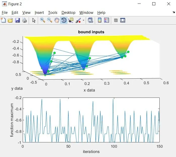
figure(2)
subplot(2,1,1);
hold on
surfc(xx,yy,f);
shading interp;
xlabel('x data')
ylabel('y data')
plot3(xopt,yopt,Fopt,'marker','o','markersize',5,'markerfacecolor','g');
title('bound inputs');

subplot(2,1,2);
plot(Fopt);
xlabel('iterations');
ylabel('function maximum');

%study3
options=optimoptions('ga');
options=optimoptions(options,'populationsize',450);
tic
for i=1:num_case
    [inputs,Fopt(i)]=ga(@stagalmite,2,[],[],[],[],[0:0],[1:1],[],[],options);
    xopt(i)=inputs(1);
    yopt(i)=inputs(2);
end
study3=toc
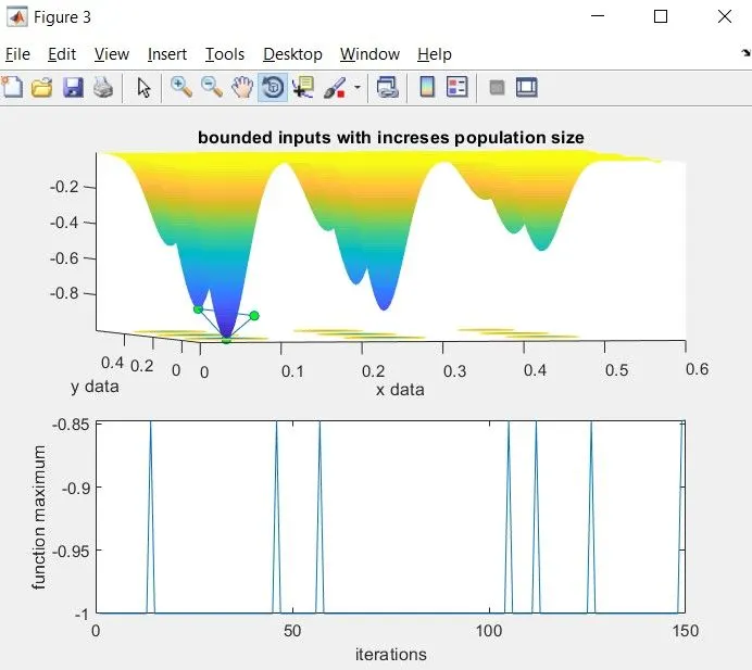
figure(3)
subplot(2,1,1);
hold on
surfc(xx,yy,f);
shading interp;
xlabel('x data')
ylabel('y data')
plot3(xopt,yopt,Fopt,'marker','o','markersize',5,'markerfacecolor','g');
title('bounded inputs with increses population size');

subplot(2,1,2);
plot(Fopt);
xlabel('iterations');
ylabel('function maximum');

max_value=Fopt

Function:

function y=stagalmite(input_vector)
    x=input_vector(1);
    y=input_vector(2);
    f1_x = (sin(5.1*pi*x+0.5))^6;
    f1_y = (sin(5.1*pi*y+0.5))^6;
    f2_x = exp(-4*log(2)*((x-0.0667)^2/0.64));
    f2_y = exp(-4*log(2)*((y-0.0667)^2/0.64)); 
    y = -[f1_x*f1_y*f2_x*f2_y];
end

Result:

Study 1:

Study 2:

Study 3:

Inference:

Thus the program to run the genetic algorithm using the stalgamite function is done. The studies are made with respect to the input bounds and population size. The graphs shows the differnce is studies and use of GA in the program.