Week 5.2 - Literature review: ODE Stability

When does a ODE become unstable?

In order to find the unstable condition for a ODE lets assume a equation for ODE and run the program for various dt.

Equation: f(y) = dy/dt = - 1000y-e^-t

For this equation we find the analytical results along with explicit and implicit methods for the result and compare one another for the stability of the profound ODE. Then program from video is used and equation is run for 0.5 seconds with various dt to find the unstable condition.

Euler Method:

In mathematics and computational science, the Euler method (also called forward Euler method) is a first-order numerical procedure for solving ordinary differential equations (ODEs) with a given initial value. It is the most basic explicit method for numerical integration of ordinary differential equations and is the simplest Runge–Kutta method. The Euler method is named after Leonhard Euler, who treated it in his book Institutionum calculi integralis. The Euler method is a first-order method, which means that the local error (error per step) is proportional to the square of the step size, and the global error (error at a given time) is proportional to the step size. The Euler method often serves as the basis to construct more complex methods, e.g., predictor–corrector method.

Explicit function : Y(k+1) = Y(k) + f(t(k),Y(k)dt

Implicit function : Y(k+1) = Y(k) + f(t(k),Y(k+1)dt

Program:

import numpy as np 
import matplotlib.pyplot as plt 
import math

def analytical(t_tot, dt):
	t = np.arange(0, t_tot, dt)
	y = np.zeros(len(t))

	for i in range(0,len(t)):
		y[i] = math.exp(-1000*t[i])*(1-math.exp(999*t[i]))/999;
	return[t,y]


def explicit(t_tot, dt):
	t = np.arange(0, t_tot, dt)
	y = np.zeros(len(t))

	for i in range(0,len(t)):
		y[i] = y[i-1] + dt*(-1000*y[i-1] - np.exp(-t[i-1]));
	return[t,y]

def implicit(t_tot, dt):
	t = np.arange(0, t_tot, dt)
	y = np.zeros(len(t))

	for i in range(0,len(t)):
		y[i] = (y[i-1] - np.exp(-t[i])*dt)/(1+1000*dt);
	return[t,y]

t_tot = 0.5
dt = 0.0005

t,y_ana = analytical(t_tot,dt)
t,y_exp = explicit(t_tot,dt)
t,y_imp = implicit(t_tot,dt)

plt.plot(t,y_ana)
plt.plot(t,y_exp)
plt.plot(t,y_imp)
plt.legend(["analytical","explicit","implicit"])
plt.grid('on')
title = ('timestep:',dt)
plt.title(title)
plt.show()

Graph:

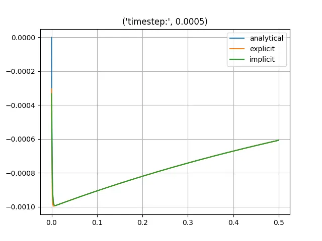
for dt = 0.0005

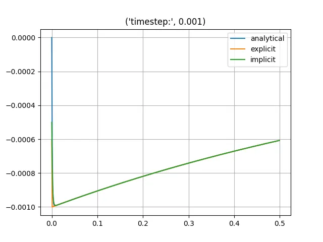
for dt = 0.001

for dt = 0.005

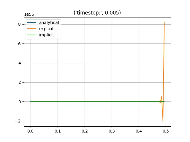
so the graphs show that the ODE is stable for small dt values. The dt of 0.001 is biggest suitable dt. thus the dt value bigger than 0.001 the ODE become unstable.

How does stability affect engineering simulations?

As far as engineering simulation are concerned stable solutions are i.e, the soltuion should reach a equailrium after certain point. Unstable solutions are characterised by large oscillations or changes in the solution wich does not die down or stabilize even after a cetain point such solutions are not at all useful in engineering simulations. If the oscilation is the soltion die down or disappears as we progress then such a solution is reliable.

Can stability condition be derived for all types of problems?

Stablity consition can only be derived for linear ode's. for the non-linear ode's it is possible by defineing a jacobian matrix. Jacobian matrix is nothing but a matrix of first order derivatives of all the functions with respect to all the independant variable. Eigen value of the jacabian matrix is computed, if all the eigen values are negative then the ode is said to be stable if one of the eigen value is positive then the solution becomes unstable.