Week 9 - Senstivity Analysis Assignment

 Sensitivity analysis:

       Sensitivity analysis is the study of how the uncertainty in the output of a mathematical model or system (numerical or otherwise) can be divided and allocated to different sources of uncertainty in its inputs. A related practice is uncertainty analysis, which has a greater focus on uncertainty quantification and propagation of uncertainty; ideally, uncertainty and sensitivity analysis should be run in tandem.

The process of recalculating outcomes under alternative assumptions to determine the impact of a variable under sensitivity analysis can be useful for a range of purposes, including:

• Testing the robustness of the results of a model or system in the presence of uncertainty.
• Increased understanding of the relationships between input and output variables in a system or model.
• Uncertainty reduction, through the identification of model input that cause significant uncertainty in the output and should therefore be the focus of attention in order to increase robustness (perhaps by further research).
• Searching for errors in the model (by encountering unexpected relationships between inputs and outputs).
• Model simplification – fixing model input that has no effect on the output, or identifying and removing redundant parts of the model structure.
• Enhancing communication from modelers to decision makers (e.g. by making recommendations more credible, understandable, compelling or persuasive).
• Finding regions in the space of input factors for which the model output is either maximum or minimum or meets some optimum criterion (see optimization and Monte Carlo filtering).
• In case of calibrating models with large number of parameters, a primary sensitivity test can ease the calibration stage by focusing on the sensitive parameters. Not knowing the sensitivity of parameters can result in time being uselessly spent on non-sensitive ones.
• To seek to identify important connections between observations, model inputs, and predictions or forecasts, leading to the development of better models.

Coding Approach:

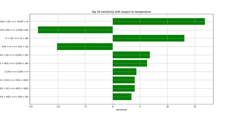
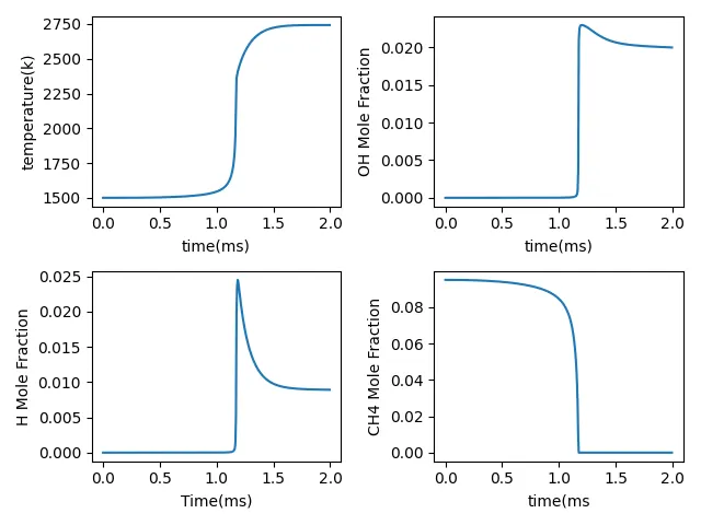
    Initially the program is written to find do sensitivity analysis for all the reaction in Methane (CH4) combustion using the source code from the video.  The number of reaction happening is found using the reaction object from gri mechanism. Then the for loop is created for the number of reaction to run sensitivity test with respect to temperature for each reaction.  Then all Reactions are needed to be sorted with to sensitivity from higher to lower sensitivity. The source coding for sorting in decending order of the sensitvity is obtained from python coding blogs and sorted the sensitvity.  Then first ten in is seperated and appended in a new varialble. Then they are ploted.  There are 325 reactions happening.  The program is written in a manner where n is variable of an int which will show the top n(int as input) and plot the graph for them. 

Program:

import numpy as np 
import cantera as ct 
import matplotlib.pyplot as plt 

gas = ct.Solution('gri30.xml')

T = 1500
P = ct.one_atm

gas.TPX = T, P,'CH4:1, O2:2, N2:7.52'

r = ct.IdealGasConstPressureReactor(gas, name = 'R1')
sim = ct.ReactorNet([r])

reac = gas.reaction_equations()

n_reac = gas.n_reactions

n = 10

S_max = [0]*n_reac

for i in range(n_reac):
	r.add_sensitivity_reaction(i)

sim.rtol = 1.0e-6
sim.atol = 1.0e-15

sim.rtol_sensitivity = 1.0e-6
sim.atol_sensitivity = 1.0e-6

states = ct.SolutionArray(gas, extra = 't')

reac_num = np.arange(1,n_reac+1)

for t in np.arange(0, 2e-3, 5e-6):
	sim.advance(t)
	states.append(r.thermo.state, t = 1000*t)

	for j in range(n_reac):
		s = sim.sensitivity('temperature', j)
		if np.abs(s)>np.abs(S_max[j]):
			S_max[j] = s

S_abs = np.abs(S_max)

reac = [a for b, a in sorted(zip(S_abs,reac), reverse=True)]
reac_num = [ a for b, a in sorted(zip(S_abs,reac_num), reverse=True)]
S_max = [a for b, a in sorted(zip(S_abs,S_max), reverse=True)]

max_r = reac[0:n]
max_n = reac_num[0:n]
max_s = S_max[0:n]

plt.figure(1)
plt.grid('on')
plt.barh(max_r, max_s, color = 'green')
plt.gca().invert_yaxis()
plt.xlabel('sensitivity')
plt.ylabel('Reactions')
plt.title('Top {} sensitivity with respect to temperature'.format(n))

plt.figure(2)
plt.subplot(2,2,1)
plt.plot(states.t, states.T)
plt.xlabel('time(ms)')
plt.ylabel('temperature(k)')
plt.subplot(2,2,2)
plt.plot(states.t, states('OH').X)
plt.xlabel('time(ms)')
plt.ylabel('OH Mole Fraction')
plt.subplot(2,2,3)
plt.plot(states.t, states('H').X)
plt.xlabel('Time(ms)')
plt.ylabel('H Mole Fraction')
plt.subplot(2,2,4)
plt.plot(states.t, states('CH4').X)
plt.xlabel('time(ms')
plt.ylabel('CH4 Mole Fraction')
plt.tight_layout()


plt.show()

Resulting Graph:

Sensitivity Bar Graph:

Molar fraction w.r.t graph:

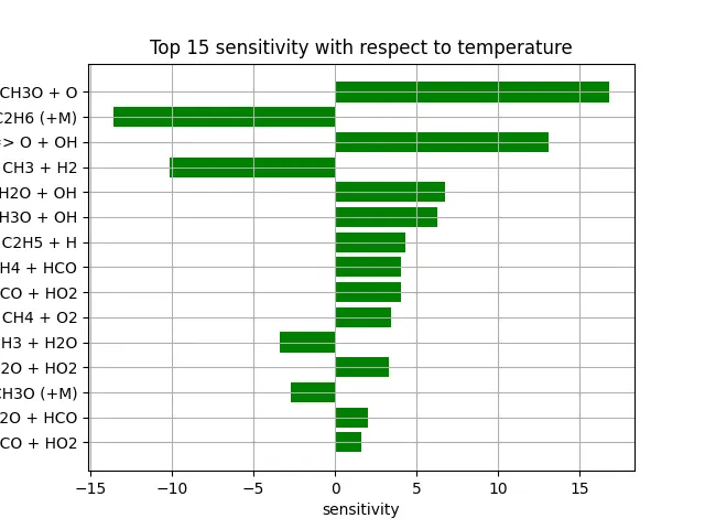
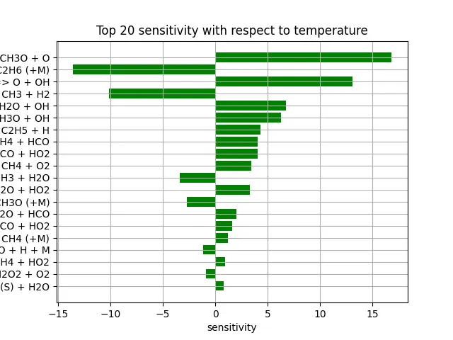
     As the per the question in the challege 'n' is variable for number reaction sensitivity to be ploted in decending order from the 325 reactions. The following graph show the result changing the n value to 15 and 20

Top 15:

Top 20:

Inference:

      From the result, it seems the oxidising reactions produce more sensitvity in temperature reducing reaction provide less sensitivity with respect to temperature.  The program and challenge was very helpful in understanding the sensitivity analysis by implementing it in combustion reaction.