Week 7 - Auto ignition using Cantera
Auto-Ignition Temperature:
The autoignition temperature or kindling point of a substance is the lowest temperature in which it spontaneously ignites in a normal atmosphere without an external source of ignition, such as a flame or spark. This temperature is required to supply the activation energy needed for combustion. The temperature at which a chemical ignites decreases as the pressure or oxygen concentration increases. It is usually applied to a combustible fuel mixture.
The ignition temperature of a substance is the least temperature at which the substance starts combustion.
Substances which spontaneously ignite in a normal atmosphere at naturally ambient temperatures are termed pyrophoric. Autoignition temperatures of liquid chemicals are typically measured using a 500-millilitre (18 imp fl oz; 17 US fl oz) flask placed in a temperature-controlled oven in accordance with the procedure described in ASTM E659.
When measured for plastics, autoignition temperature can be also measured under elevated pressure and at 100% oxygen concentration. The resulting value is used as a predictor of viability for high-oxygen service. The main testing standard for this is ASTM G72.
Auto-ignition equation:
The time it takes for a material to reach its autoignition temperature when exposed to a heat flux  is given by the following equation

where k = thermal conductivity, ρ = density, and c = specific heat capacity of the material of interest,  is the initial temperature of the material (or the temperature of the bulk material).
Coding Approch:
A basic function that suits all the cases for the question is created using the reactor network reference code to stimulate the Auto-Ignition for methane.
Basic Function Program:
def cv_combust(T,P,species_dict):
	gas = ct.Solution('gri30.xml')
	gas.TPX = T, P*ct.one_atm, species_dict

	r = ct.IdealGasReactor(gas)
	sim = ct.ReactorNet([r])
	time = 0.0
	states = ct.SolutionArray(gas, extra = ['time_in_ms','t'])

	Time_start = 0
	time_end = 1
	dt = 1e-3
	n = int((time_end - Time_start)/dt)

	for n in range(n):
		time += 1e-3
		sim.advance(time)
		states.append(r.thermo.state,time_in_ms = time*1e-3, t=time)
		print (states.T)
		print (states.time_in_ms)
	plt.plot(states.T, states.time_in_ms)
	plt.show()
	plt.grid('on')
	return states
Then using the formula for ignition time.
To find the ignition time, The formula is implemented in the basic function for auto-ignition stimulation.
T_check = states.T[i] - T - 400
if T_check>0:
	temperature_auto_ignition = states.T[i]
	time_auto_ignition = states.time_in_ms[i]
	break
Since the basic function is created properly, a range of input is changed with the cases provided to problem to solve.
Auto-ignition time of Methane:
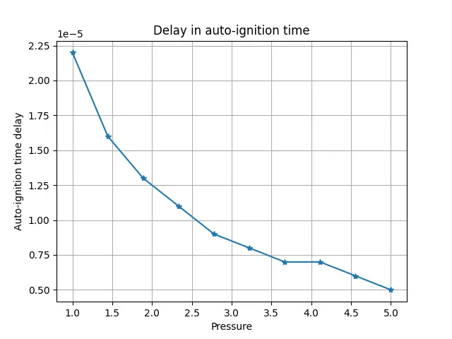
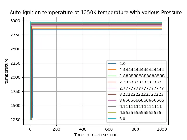
Case 1: Temperature = 1250K; Pressure= 1 to 5 Bar.
Program:
import sys
import numpy as np
import matplotlib.pyplot as plt
import cantera as ct

Pressure = np.linspace(1,5,10)
T = 1250
species_dict = {'CH4':1, 'O2':2, 'N2':7.52}
auto_ignition_delay_P = []
state_T = []

def cv_combust(T,P,species_dict):
	gas = ct.Solution('gri30.xml')
	gas.TPX = T, P*ct.one_atm, species_dict

	r = ct.IdealGasReactor(gas)
	sim = ct.ReactorNet([r])
	time = 0.0
	states = ct.SolutionArray(gas, extra = ['time_in_ms','t'])

	Time_start = 0
	time_end = 10
	dt = 1e-3
	n = int((time_end - Time_start)/dt)

	for n in range(n):
		time += 1e-3
		sim.advance(time)
		states.append(r.thermo.state,time_in_ms = time*1e-3, t=time)
		print (states.T)
		print (states.time_in_ms)
	for i in range(n):
		T_check = states.T[i] - T - 400
		if T_check>0:
			temperature_auto_ignition = states.T[i]
			time_auto_ignition = states.time_in_ms[i]
			break
	auto_ignition_delay_P.append(time_auto_ignition)

	return states

for P in Pressure:
	states = cv_combust(T,P,species_dict)
	state_T.append(states.T)

state_T = np.array(state_T)

print (auto_ignition_delay_P)

print (Pressure)

plt.figure(1)
plt.plot(Pressure,auto_ignition_delay_P,'-*')
plt.xlabel('Pressure')
plt.ylabel('Auto-ignition time delay')
plt.grid('on')
plt.title('Delay in auto-ignition time')


state_T = np.array(state_T)
print(state_T)
for k in range(len(Pressure)):
	plt.figure(2)
	LP = Pressure[k]
	plt.plot(state_T[k],label = str(LP))
	plt.xlabel('Time in micro second')
	plt.ylabel('temperature')
	plt.grid('on')
	plt.title('Auto-ignition temperature at 1250K temperature with various Pressure')
	plt.legend()


plt.show()
Resulting Graph:
Auto-ignition delay:
Auto-ignition Temperature:
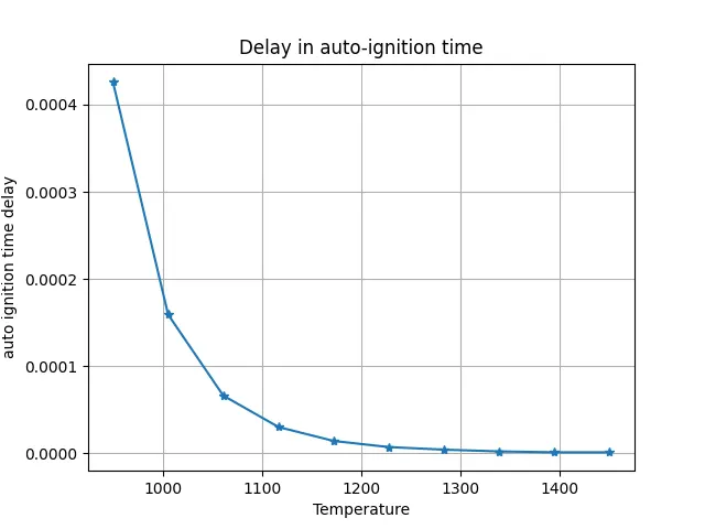
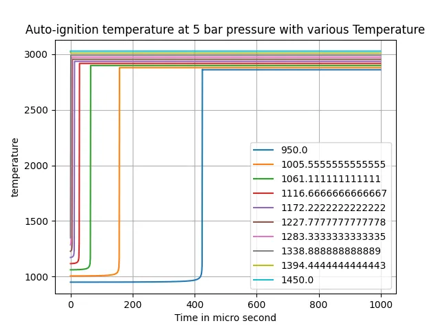
Case: Temperature = 950K to 1450K; Pressure= 5 Bar.
Program:
import sys
import numpy as np
import matplotlib.pyplot as plt
import cantera as ct

P = 5
Temperature = np.linspace(950,1450,10)
species_dict = {'CH4':1, 'O2':2, 'N2':7.52}
auto_ignition_delay_P = []
state_T = []


def cv_combust(T,P,species_dict):
	gas = ct.Solution('gri30.xml')
	gas.TPX = T, P*ct.one_atm, species_dict

	r = ct.IdealGasReactor(gas)
	sim = ct.ReactorNet([r])
	time = 0.0
	states = ct.SolutionArray(gas, extra = ['time_in_ms','t'])

	Time_start = 0
	time_end = 10
	dt = 1e-3
	n = int((time_end - Time_start)/dt)

	for n in range(n):
		time += 1e-3
		sim.advance(time)
		states.append(r.thermo.state,time_in_ms = time*1e-3, t=time)
		print (states.T)
		print (states.time_in_ms)
	for i in range(n):
		T_check = states.T[i] - T - 400
		if T_check>0:
			temperature_auto_ignition = states.T[i]
			time_auto_ignition = states.time_in_ms[i]
			break
	auto_ignition_delay_P.append(time_auto_ignition)

	return states

for T in Temperature:
	states = cv_combust(T,P,species_dict)
	state_T.append(states.T)

state_T = np.array(state_T)

print (auto_ignition_delay_P)

print (Temperature)

plt.plot(Temperature,auto_ignition_delay_P,'-*')
plt.xlabel('Temperature')
plt.ylabel('auto ignition time delay')
plt.grid('on')
plt.title('Delay in auto-ignition time')

state_T = np.array(state_T)
print(state_T)
for k in range(len(Temperature)):
	plt.figure(2)
	LT = Temperature[k]
	plt.plot(state_T[k], label = str(LT))
	plt.xlabel('Time in micro second')
	plt.ylabel('temperature')
	plt.grid('on')
	plt.title('Auto-ignition temperature at 5 bar pressure with various Temperature')
	plt.legend()


plt.show()
Resulting Graph:
Auto-Ignition Delay:
Auto-ignition Temperature:
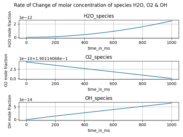
Part -2: Rate of Change of molar concentration.
Case 1:Temperature is 1000K and pressure 5 bar
Program:
import sys
import numpy as np
import matplotlib.pyplot as plt
import cantera as ct

P = 5
T = 1000
species_dict = {'CH4':1, 'O2':2, 'N2':7.52}

def cv_combust(T,P,species_dict):
	gas = ct.Solution('gri30.xml')
	gas.TPX = T, P, species_dict

	r = ct.IdealGasReactor(gas)
	sim = ct.ReactorNet([r])
	time = 0.0
	states = ct.SolutionArray(gas, extra = ['time_in_ms','t'])

	Time_start = 0
	time_end = 10
	dt = 1e-3
	n = int((time_end - Time_start)/dt)

	for n in range(1000):
		time += 1e-3
		sim.advance(time)
		states.append(r.thermo.state,time_in_ms = time*1e-3, t=time)
	H2O_species = states.X[:,gas.species_index('H2O')]
	O2_species = states.X[:,gas.species_index('O2')]
	OH_species = states.X[:,gas.species_index('OH')]


	return [states,H2O_species,O2_species,OH_species]

states,H2O_species,O2_species,OH_species = cv_combust(T,P,species_dict)
print(H2O_species)
print(O2_species)
print(OH_species)

fig, ax = plt.subplots(3)

ax[0].plot(H2O_species)
ax[0].set_title('H2O_species')
ax[0].set_xlabel('time_in_ms')
ax[0].set_ylabel('H2O mole fraction')
ax[0].grid('on')

fig.suptitle("Rate of Change of molar concentration of species H2O, O2 & OH ")

ax[1].plot(O2_species)
ax[1].set_title('O2_species')
ax[1].set_xlabel('time_in_ms')
ax[1].set_ylabel('O2 mole fraction')
ax[1].grid('on')

ax[2].plot(OH_species)
ax[2].set_title('OH_species')
ax[2].set_xlabel('time_in_ms')
ax[2].set_ylabel('OH mole fraction')
ax[2].grid('on')

fig.tight_layout()
plt.show()
Resulting Graph:
Case 2: Temperature is 500K and pressure 5 bar
Program:
import sys
import numpy as np
import matplotlib.pyplot as plt
import cantera as ct

P = 5
T = 500
species_dict = {'CH4':1, 'O2':2, 'N2':7.52}

def cv_combust(T,P,species_dict):
	gas = ct.Solution('gri30.xml')
	gas.TPX = T, P, species_dict

	r = ct.IdealGasReactor(gas)
	sim = ct.ReactorNet([r])
	time = 0.0
	states = ct.SolutionArray(gas, extra = ['time_in_ms','t'])

	Time_start = 0
	time_end = 10
	dt = 1e-3
	n = int((time_end - Time_start)/dt)

	for n in range(1000):
		time += 1e-3
		sim.advance(time)
		states.append(r.thermo.state,time_in_ms = time*1e-3, t=time)
	H2O_species = states.X[:,gas.species_index('H2O')]
	O2_species = states.X[:,gas.species_index('O2')]
	OH_species = states.X[:,gas.species_index('OH')]


	return [states,H2O_species,O2_species,OH_species]

states,H2O_species,O2_species,OH_species = cv_combust(T,P,species_dict)
print(H2O_species)
print(O2_species)
print(OH_species)

fig, ax = plt.subplots(3)

ax[0].plot(H2O_species)
ax[0].set_title('H2O_species')
ax[0].set_xlabel('time_in_ms')
ax[0].set_ylabel('H2O mole fraction')
ax[0].grid('on')

fig.suptitle("Rate of Change of molar concentration of species H2O, O2 & OH ")

ax[1].plot(O2_species)
ax[1].set_title('O2_species')
ax[1].set_xlabel('time_in_ms')
ax[1].set_ylabel('O2 mole fraction')
ax[1].grid('on')

ax[2].plot(OH_species)
ax[2].set_title('OH_species')
ax[2].set_xlabel('time_in_ms')
ax[2].set_ylabel('OH mole fraction')
ax[2].grid('on')

fig.tight_layout()
plt.show()
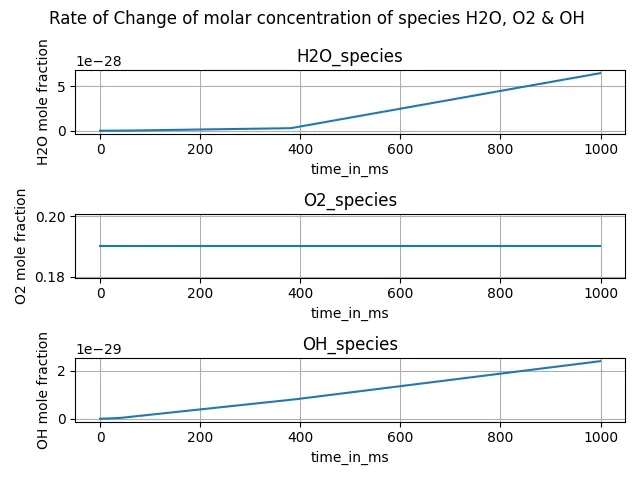
Resulting Graph:
Inference:
From the Auto-Ignition stimulation done, it is studied that the Increase in Temperature or the Pressure reduces the auto-ignition time delay i.e. the higher the temperature or pressure the lesser micro-seconds it need to auto-ignite. The auto-ignition temperature also is higher when there is high Initial temperature and pressure. Thus the higher the initial temperature or pressure it affects the auto-ignition significantly in delay time and ingnition temprature.
Then in the second part of the problem the molar fraction of the species like water, oxygen and hydroxide molecules changes studied in the graph show the auto-ignition of the fuel with that initial conditon.