Week 5 - Rayleigh Taylor Instability
Rayleigh taylor instability
The Rayleigh–Taylor instability, or RT instability (after Lord Rayleigh and G I Taylor), is an instability of an interface between two fluids of different densities which occurs when the lighter fluid is pushing the heavier fluid. Examples include the behavior of water suspended above oil, Mushroom clouds like those from volcanic erruptions and atmospheric Nuclear explosions,Supernova explosions in which expanding core gas is accelerated into denser shell gas, instabilities in plasma fusion reactors and inertial confinement fusion.
Types of Instabilities
1. Ritchmyer-Meshkov
2. Plateau Rayleigh
3. Kelvin Helmholts
Ritchmyer-Meshkov
The Richtmyer–Meshkov instability (RMI) occurs when two fluids of different density are impulsively accelerated. Normally this is by the passage of a shocl wave. The development of the instability begins with small amplitude perturbations which initially grow linearly with time. This is followed by a nonlinear regime with bubbles appearing in the case of a light fluid penetrating a heavy fluid, and with spikes appearing in the case of a heavy fluid penetrating a light fluid. A chaotic regime eventually is reached and the two fluids mix. This instability can be considered the impulsive-acceleration limit of the RTI.
Plateau Rayleigh
The Plateau–Rayleigh instability, often just called the Rayleigh instability, explains why and how a falling stream of fluid breaks up into smaller packets with the same volume but less surface area. It is related to the RTI and is part of a greater branch of fluid dynamics concerned with fluid thread breakup. This fluid instability is exploited in the design of a particular type of ink jet technology whereby a jet of liquid is perturbed into a steady stream of droplets.
The driving force of the Plateau–Rayleigh instability is that liquids, by virtue of their surface tensions, tend to minimize their surface area. A considerable amount of work has been done recently on the final pinching profile by attacking it with self similar solutions.
Kelvin Helmholts
The Kelvin–Helmholtz instability (after Lord Kelvin and Hermann von Helmholtz) typically occurs when there is velocity shear in a single continous fluid, or additionally where there is a velocity difference across the interface between two fluids. A common example is seen when wind blows across a water surface; the instability constant manifests as waves. Kelvin-Helmholtz instabilities are also visible in the atmospheres of planets and moons, such as in cloud formations on Earth or the Red Spot on jupiter , and the atmospheres (coronas) of stars, including the sun's.
Practical CFD models based on instability
1. Smoothed Particle Hydrodynamics
2. Single Fluid Model
3. Two-Fluid Model
4. Turbulence Model
Smoothed Particle Hydrodynamics
Smoothed-particle hydrodynamics (SPH) is a computational method used for simulating the mechanics of continuum media, such as solid Mechanics and Fluid flows. It was developed by Gingold and Monagan and Lucy in 1977, initially for astrophysical problems. It has been used in many fields of research, including Astrophysics, ballistics, volcanology, and oceanography. It is a meshfree Lagrangian Method(where the co-ordinates move with the fluid), and the resolution of the method can easily be adjusted with respect to variables such as Density.
Two-Fluid Model
In the two-fluid model, a set of conservation equations for mass, momentum and energy is solved for each phase (Ishii and Hibiki, 2006). As a consequence of the time averaging procedure, the detailed structure of the interphase is lost and, therefore, interphase exchanges of mass, momentum and energy need to be modelled. In the momentum equation, the drag force, lift force, wall force and turbulent dispersion force contribute to the momentum interphase transfer. Turbulence is solved in the continuous phase only with a multiphase Reynolds stress formulation based on the SSG model (Speziale et al., 1991). The dispersed phase turbulence is then directly related to that of the continuous phase.
Turbulence Model
Turbulence modeling is the construction and use of a mathemaatical model to predict the effects of turbulence. Turbulent flows are commonplace in most real life scenarios, including the flow of blood through the cardiovascular system, the airflow over an aircraft wing, the re-entry of space vehicles, besides others. In spite of decades of research, there is no analytical theory to predict the evolution of these turbulent flows. The equations governing turbulent flows can only be solved directly for simple cases of flow. For most real life turbulent flows, CFD simulations use turbulent models to predict the evolution of turbulence. These turbulence models are simplified constitutive equations that predict the statistical evolution of turbulent flows
SIMULATION
Geometry
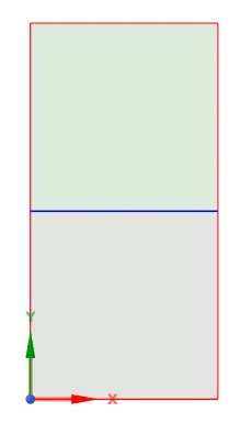
Measurements 20mmX20mm for each square.
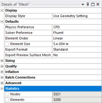
Mesh profile : base mesh with mesh size 0.5mm
no of nodes : 3321
no of elements : 3200
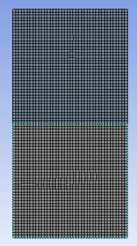
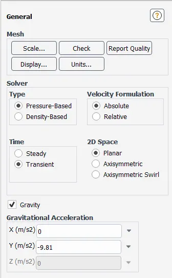
Pressure based transient solver used. We use the transient setting as we have to capture the physics and details at each time step as there will be minute changes with respect to time.
We have also enabked gravity as it plays an important role in fluid simulation like this.
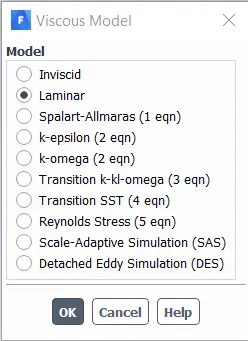 viscous model used here is Laminar as we are not dealing with flow velocities which generates turbulence in the simulation.
Also we have Multiphase physics enabled.
In the Euler-Euler approach, the different phases are treated mathematically as interpenetrating continua. Since the volume of a phase cannot be occupied by the other phases, the concept of phasic volume fraction is introduced. These volume fractions are assumed to be continuous functions of space and time and their sum is equal to one. Conservation equations for each phase are derived to obtain a set of equations, which have similar structure for all phases. These equations are closed by providing constitutive relations that are obtained from empirical information, or, in the case of granular flows , by application of kinetic theory.
In ANSYS FLUENT, three different Euler-Euler multiphase models are available: the volume of fluid (VOF) model, the mixture model, and the Eulerian model.
The VOF Model
The VOF model is a surface-tracking technique applied to a fixed Eulerian mesh. It is designed for two or more immiscible fluids where the position of the interface between the fluids is of interest. In the VOF model, a single set of momentum equations is shared by the fluids, and the volume fraction of each of the fluids in each computational cell is tracked throughout the domain. Applications of the VOF model include stratified flows , free-surface flows, filling, sloshing , the motion of large bubbles in a liquid, the motion of liquid after a dam break, the prediction of jet breakup (surface tension), and the steady or transient tracking of any liquid-gas interface.
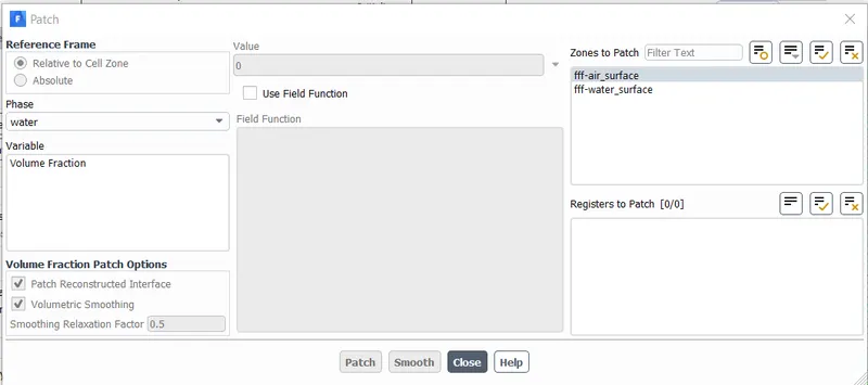
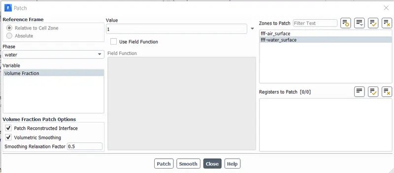
so here, we have to patch the 2 fluids. Patch condition contains no geometric or topological information about mesh. Typically patch is used for an inlet or an outlet. symmetryPlane. Symmetry plane (mirroring quantity)
we give the value 0 for air surface and value 1 for the water. we patch this interface because we define that there is a mix going to happen between the two fluids.
 .
.
After patching is done we then calcuate the solution and run it. after which the results are obtained.
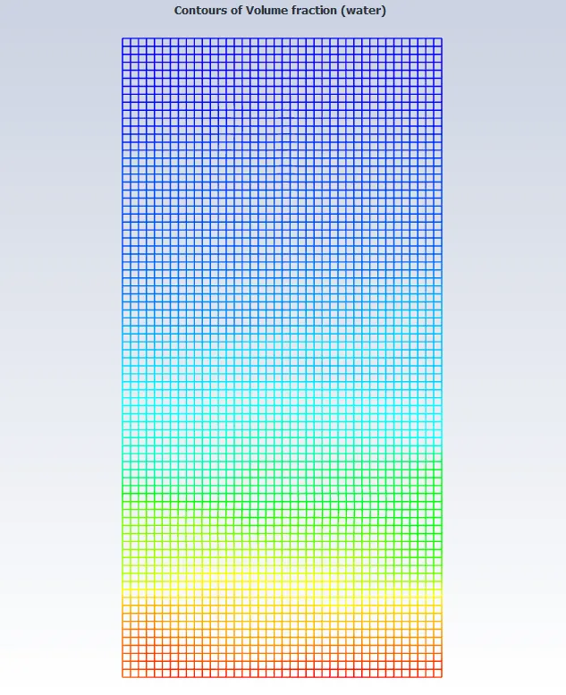
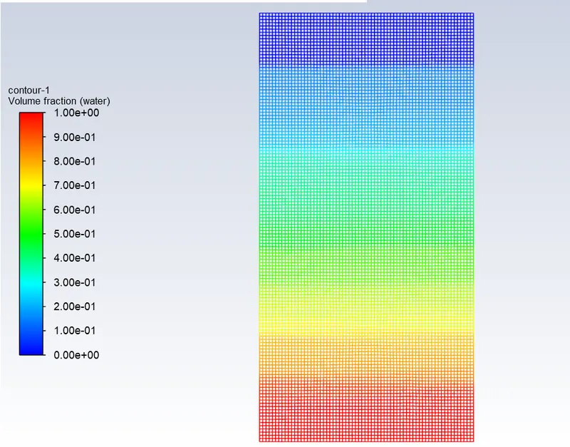
Contour for all three would be graphically the same as every case reaches an equilibrium in its state.
Below you can find the youtube links to the simulations
case 1
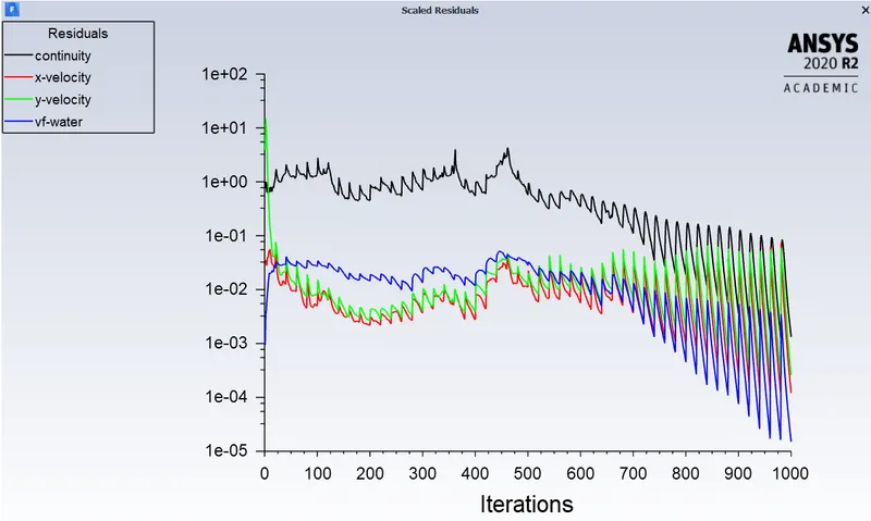
This is the first case, here the element size is 0.5mm for mesh. Here you can see equilibrium state reaches quite fast compared to the other two cases. This is mainly because of the coarse mesh profile.
Finer the mesh gets, more physics and data can be captured and simulation time will be increased.
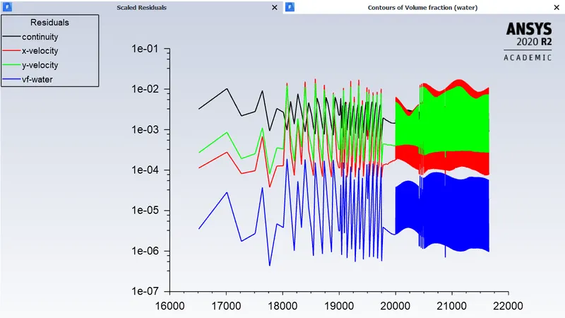
Residual plot
Case 2
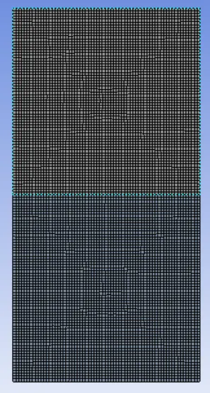
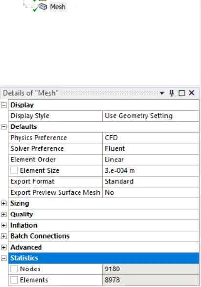
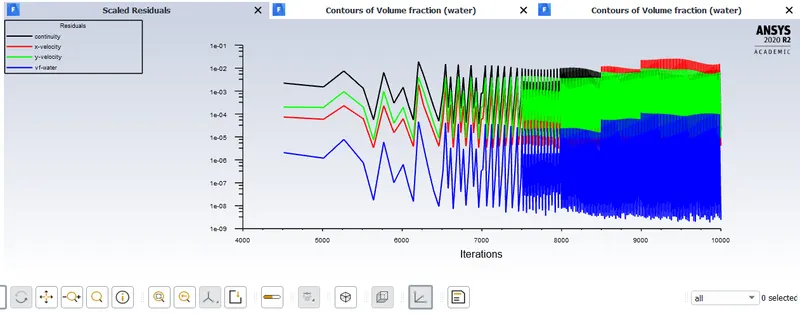
Here base mesh value is 0.3mm and then same setup and boundary conditions. Here you can see the difference where more of the physics is captured at each time step.
Mesh profile
residuals
case 3
Mesh element would be 0.3mm, same as case 2.
Here we use a User defined fluid with visc = 400 `(Kg)/m^3`
and density = 0.001 `(Kg)/(m s)`
residuals
final contour plot for case 3
ATWOOD number.
The Atwood number (A) is a dimensionless number in fluid dynamics used in the study of hydrodynamic instabilities in density stratified flows. It is a dimensionless density ratio defined as

where
 = density of heavier fluid
 = density of lighter fluid
- Atwood number is an important parameter in the study of Rayleigh–Taylor instability and Richtmyer–Meshkov instability. In Rayleigh–Taylor instability, the penetration distance of heavy fluid bubbles into the light fluid is a function of acceleration time scale,
 where g is the gravitational acceleration and t is the time.
 - That is why we are activating the gravity in y direction.
Case 1
`rho`1 = 997 `(kg)/(m^3)`
`rho`2 = 1.225 `(kg)/(m^3)`
A = 0.9975.
The value is same for case two as only the mesh profile and element size is changed.
Case 3
`rho`1 = 997 water
ρ2 = 400 user defined fluid
A = 0.427.
Now when the Atwood number is closer to 1, plume like structures form when a heavy fluid is mixed to a light fluid.
And when the atwood number is closer to 0, we see finger like structures forming at the interface.
Smaller Atwood numbers result in longer delay distances. Higher Atwood numbers shorten the delay and its associated distance, providing a longer development period for the R–T mixing.
Atwood number, abbreviated as A, a dimensionless number, describes density difference between two adjacent fluids with a common interface.
The Reason we used the Transient solver is because we need to understand what is aheppening at every instant of the simulation. If we use the steady state solver, we know that eventually these two fluids come to equilibrium and we dont need only the last results.