Week 7 - Simulation of a 1D Super-sonic nozzle flow simulation using Macormack Method
TITLE
1D flow through a convergent divergent nozzle(subsonic-supersonic)
OBJECTIVES
To show the steady state distribution of primitive variables in the nozzle
2. Time-wise variation of the primitive variables
3. Variation of Mass flow rate distribution inside the nozzle at different time steps during the time-marching process
4. Comparison of Normalized mass flow rate distributions of both forms
THEORY
Subsonic-supersonic(delaval or convergent-divergent nozzle) Nozzle
This nozzle has 3 main sections
a. subsonic or inlet
b. throat
c. supersonic or outlet
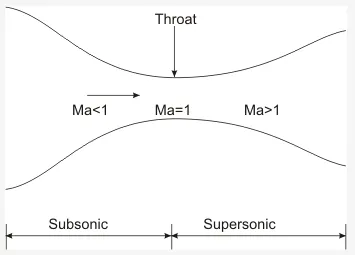
The criteria for determination of the flow, whether its subsonic or super sonic depends on the Mach number.
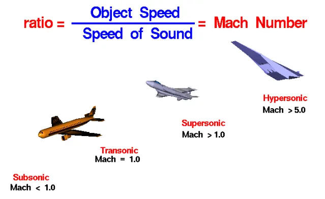
- Subsonic conditions occur for Mach numbers less than one, M < 1 . For the lowest subsonic conditions, compressibility can be ignored.
- As the speed of the object approaches the speed of sound, the flight Mach number is nearly equal to one, M = 1, and the flow is said to be transonic. At some places on the object, the local speed exceeds the speed of sound. Compressibility effects are most important in transonic flows and lead to the early belief in a sound barrier. Flight faster than sound was thought to be impossible. In fact, the sound barrier was only an increase in the drag near sonic conditions because of compressibility effects. Because of the high drag associated with compressibility effects, aircraft do not cruise near Mach 1.
- Supersonic conditions occur for Mach numbers greater than one, 1 < M < 3. Compressibility effects are important for supersonic aircraft, and shock waves are generated by the surface of the object. For high supersonic speeds, 3 < M < 5, aerodynamic heating also becomes very important for aircraft design.
THEORY
There are two approaches to get this done, Conservative and Non Conservative
NON CONSERVATIVE

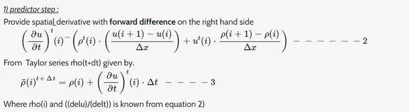
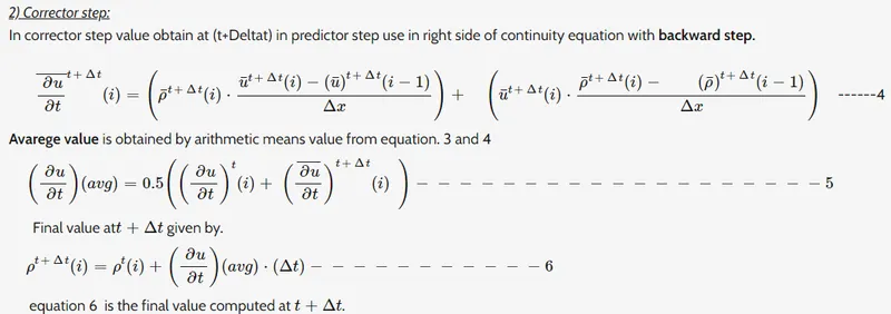
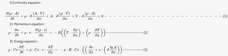
In the above equations above are in the form of dimensional numbers. But in CFD e are using non dimensional numbers which give us a better final result. Where (P/`P_0`) and (T/`T_0`) values varies from 0 to 1.
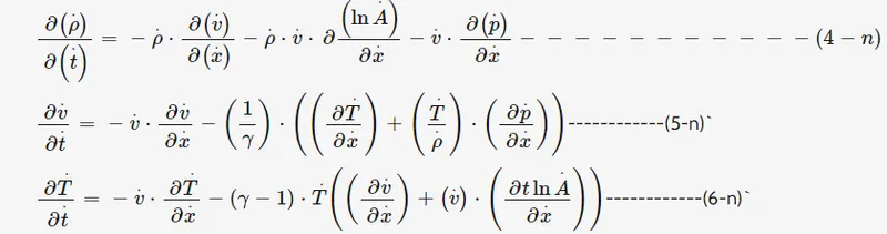
The image below shows the non dimensional multiplied on both sides of the above equations
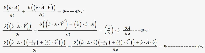
Governing equations for conservative form
 \
\
definition of the above equation with solution vector U :
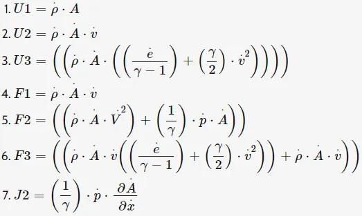
above equations can be written as
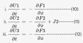
We apply the macormack's technique to solve the problem and get solutions.
To obtain the primitive variables we need to decode variables u1 u2 and u3 and we use those values to find out primitive variables
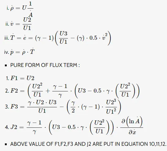
For Non Conservative form
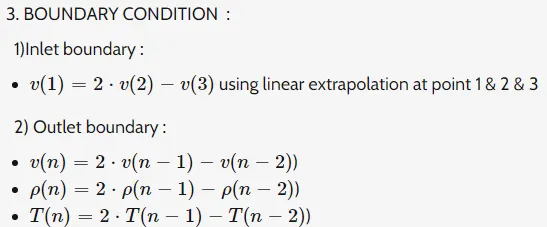
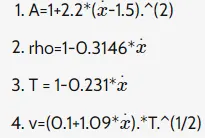
Initial Conditions(same for both forms)
Boundary conditions for Conservative
INLET
u1(1)=a(1);
u2(1)=2*u2(2)-u2(3);
v_c(1) = u2(1)/u1(1);
u3(1)=u1(1)*((temp_c(1)/(gamma-1)) + 0.7*(v_c(1)^2));
OUTLET
u1(n)=2*u1(n-1)-u1(n-2);
u2(n)=2*u2(n-1)-u2(n-2);
u3(n)=2*u3(n-1)-u3(n-2);
CODE LOGIC
CODE
clear all
close all
clc

nt=1400;
% calling non conservative function
tic
[v,rho,temp,m,mach_no,p,rho_t,v_t,temp_t,p_t,mach_no_t,m_t,x]=nozzle_nonconservative();
non_conservative=toc;

% calling conservative function
tic
[v_c,rho_c,temp_c,m_c,mach_no_c,p_c,rho_ct,v_ct,temp_ct,p_ct,mach_no_ct,m_ct]=nozzle_conservative();
conservative=toc;

%plotting conservative vs non conservative
%mass flow rate
figure(3)
subplot(3,2,1)
plot(x,m);
hold on
plot(x,m_c,'*');
%analytical solution is 0.579
a=0.579*ones(1,31);
plot(x,a,'-');
xlabel('non-dimensional flow throw the nozzle (x)');
ylabel('non-dimensional mass flow throw the nozzle (m)');
legend('non-conservative','conserative','analytical');
title('mass flow rate comparison');
grid on

%variation of non dimentional flow parameters
%mach number
subplot(3,2,2)
plot(x,mach_no);
hold on
plot(x,mach_no_c,'*');
xlabel('nozzle distace');
ylabel('mach number');
legend('non-conservative','conserative');
title('mach number comparison');
grid on

%pressure
subplot(3,2,3)
plot(x,p);
hold on
plot(x,p_c,'*');
xlabel('nozzle distace');
ylabel('presssure');
legend('non-conservative','conserative');
title('pressure comparison');
grid on

%density
subplot(3,2,4)
plot(x,rho);
hold on
plot(x,rho_c,'*');
xlabel('nozzle distace');
ylabel('density');
legend('non-conservative','conserative');
title('density comparison');
grid on

%temperature
subplot(3,2,5)
plot(x,temp);
hold on
plot(x,temp_c,'*');
xlabel('nozzle distace');
ylabel('temperature');
legend('non-conservative','conserative');
title('temperature comparison');
grid on

%velocity
subplot(3,2,6)
plot(x,v);
hold on
plot(x,v_c,'*');
xlabel('nozzle distace');
ylabel('velocity');
legend('non-conservative','conserative');
title('velocity comparison');
grid on

% variation of flow at throat
figure(4)
%plotting density
subplot(4,1,1)
plot(rho_t)
hold on
plot(rho_ct,'r')
ylabel('density');
legend('non-conservative','conserative');
title('density comparison at throat for various time step ');


%plotting temperature
subplot(4,1,2)
plot(temp_t)
hold on
plot(temp_ct,'r')
ylabel('temperature');
legend('non-conservative','conserative');
title('temperature comparison at throat for various time step ');

%pressure
subplot(4,1,3)
plot(p_t)
hold on
plot(p_ct,'r')
ylabel('pressure');
legend('non-conservative','conserative');
title('pressure comparison at throat for various time step ');

%mach number
subplot(4,1,4)
plot(mach_no_t)
hold on
plot(mach_no_ct,'r')
ylabel('mach number');
legend('non-conservative','conserative');
title('mach number comparison at throat for various time step ');
FUNCTIONS
function [v,rho,temp,m,mach_no,p,rho_t,v_t,temp_t,p_t,mach_no_t,m_t,x]=nozzle_nonconservative()
%non conservative approach
%inputs
n=31;
x=linspace(0,3,n);
dx=x(2)-x(1);

%calculating initial profiles
rho=1-0.3146*x; %density
temp= 1-0.2314*x; % temperature
v=(0.1+1.09*x).*temp.^0.5;% velocity
gamma =1.4;

a=1 + 2.2.*(x-1.5).^2;
c=0.5; %cfl condition for stability
nt=1400;
l=[1:1400];
throat=(n+1)/2;
dt=min(c.*(dx./(sqrt(temp)+v)));
% dt=0.02;
%outer time loop
for k=1:nt

    rho_old=rho;
    v_old=v;
    temp_old=temp;
    %predictor method
    for j=2:n-1
       %drho_dt_p = -rho(j)*(v(j+1)-v(j))/dx - rho(j)*v(j)*(log(a(j+1))-log(a(j)))/dx-v(j)*(rho(j).....)
        dvdx=(v(j+1)-v(j))/dx;
        drhodx=(rho(j+1)-rho(j))/dx;
        dtdx=(temp(j+1)-temp(j))/dx;
        dlogadx=(log(a(j+1))-log(a(j)))/dx;
        %continuity equation
        drhodt_p(j) = -rho(j)*dvdx -rho(j)*v(j)*dlogadx-v(j)*drhodx;

        %momentum equation
        dvdt_p(j) =-v(j)*dvdx -(1/gamma)*(dtdx+(temp(j)/rho(j))*drhodx);

        %energy equation
        dtdt_p(j)=-v(j)*dtdx-(gamma-1)*temp(j)*(dvdx+v(j)*dlogadx);

        %solution update
        rho(j)=rho(j)+drhodt_p(j)*dt;
        v(j)=v(j)+dvdt_p(j)*dt  ;
        temp(j)=temp(j)+dtdt_p(j)*dt;

    end

        %corrector method
    for j=2:n-1
       %drho_dt_p = -rho(j)*(v(j+1)-v(j))/dx - rho(j)*v(j)*(log(a(j+1))-log(a(j)))/dx-v(j)*(rho(j).....)
        dvdx=(v(j)-v(j-1))/dx;
        drhodx=(rho(j)-rho(j-1))/dx;
        dtdx=(temp(j)-temp(j-1))/dx;
        dlogadx=(log(a(j))-log(a(j-1)))/dx;
        %continuity equation
        drhodt_c(j) = -rho(j)*dvdx -rho(j)*v(j)*dlogadx-v(j)*drhodx;

        %momentum equation
        dvdt_c(j) =-v(j)*dvdx -(1/gamma)*(dtdx+(temp(j)/rho(j))*drhodx);

        %energy equation
        dtdt_c(j)=-v(j)*dtdx-(gamma-1)*temp(j)*(dvdx+v(j)*dlogadx);

    end
    %computing the average time derivative
    dvdt= 0.5*(dvdt_p + dvdt_c);
    drhodt= 0.5*(drhodt_p + drhodt_c);
    dtdt= 0.5*(dtdt_p + dtdt_c);

    %calculating residual
    dvdt_t(k)=abs(dvdt(throat));
    drhodt_t(k)=abs(drhodt(throat));
    dtdt_t(k)=abs(dtdt(throat));

    %final solution update

    for i=2:n-1
        v(i)=v_old(i)+dvdt(i)*dt;
        rho(i)=rho_old(i)+drhodt(i)*dt;
        temp(i)=temp_old(i)+dtdt(i)*dt;
    end
    %applying boundary conditions
    %inlet
    v(1)=2*v(2)-v(3);

    %outlet
    v(n)=2*v(n-1)-v(n-2);
    rho(n)=2*rho(n-1)-rho(n-2);
    temp(n)=2*temp(n-1)-temp(n-2);

    %mass flow rate m
    m=rho.*a.*v;
    %pressure ratio
    p=rho.*temp;
    %mach no
    mach_no = v./sqrt(temp);

    %VALUEs at throat
    rho_t(k)=rho(throat);
    v_t(k)=v(throat);
    temp_t(k)=temp(throat);
    p_t(k)=p(throat);
    mach_no_t(k)=  mach_no(throat);
    m_t(k)=m(throat);

    %plotting mass flow rate at different time steps
    figure(1);
    if k==50
        plot(x,m,'color','b','linewidth',1.5);
        hold on
    elseif k == 100
        plot(x,m,'color','g','linewidth',1.5);
        hold on
    elseif k == 150
        plot(x,m,'color','y','linewidth',1.5);
        hold on
    elseif k == 200
        plot(x,m,'color','black','linewidth',1.5);
        hold on
    elseif k == 500
        plot(x,m,'color','cyan','linewidth',1.5);
        hold on
    elseif k == 700
        plot(x,m,'color','r','linewidth',1.5);
        hold on
    elseif k == 1400
        plot(x,m,'color','m','linewidth',1.5);
        grid on
        title('Non Conservative')
    end
end
hold off
% 'Name','Mass flow rate at diff time step'
xlabel('non-dimensional flow throw the nozzle (x)');
ylabel('non-dimensional mass flow throw the nozzle (m)');
legend({'50 time steps','100 time steps','150 time steps','200 time steps','500 time steps','700 time steps','1400 time steps'});

figure(5)
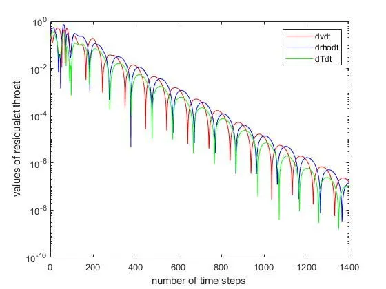
semilogy(l,dvdt_t,'r');
hold on
semilogy(l,drhodt_t,'b');
semilogy(l,dtdt_t,'g');
xlabel('number of time steps ');
ylabel('values of residual at throat');
legend('dvdt','drhodt','dTdt');

title('Non conservative')


end
Function Conservative
function [v_c,rho_c,temp_c,m_c,mach_no_c,p_c,rho_ct,v_ct,temp_ct,p_ct,mach_no_ct,m_ct]=nozzle_conservative()
% conservative approach
%inputs
n=31;
x=linspace(0,3,n);
dx=x(2)-x(1);
l=[1:1400];
%calculating initial profiles
%initialising density and temperature for conservative form.
for i=1:length(x)
    if x(i)>=0 && x(i)<=0.5
        rho_c(i)=1;
        temp_c(i)=1;
    elseif x(i)>0.5 && x(i)<=1.5
        rho_c(i)= 1-0.366*(x(i)-0.5);
        temp_c(i)=1-0.167*(x(i)-0.5);
    elseif x(i)>1.5 && x(i)<=3
        rho_c(i)= 0.634-0.3879*(x(i)-1.5);
        temp_c(i)=0.833-0.3507*(x(i)-1.5);
    end
end


gamma =1.4;
a=1 + (2.2.*((x-1.5).^2)); % nozzle area
c=0.5; %cfl condition for stability
nt=1400; % no of time steps
throat=(n+1)/2;
v_c=0.59./(rho_c.*a);% velocity
for i=1:n
    dt_calc(i) = c.*(dx./(sqrt(temp_c(i))+v_c(i)));
end
dt= min(dt_calc);
%dt = 0.0267;


%solution vector in terms of initial condition
u1= rho_c.*a;
u2= rho_c.*a.*v_c;
u3= rho_c.*((temp_c./(gamma-1))+(gamma./2)*(v_c.^2))    .*a;


 for k=1:1400
   % storing the old values of u1, u2 and u3
    u1_old=u1;
    u2_old=u2;
    u3_old=u3;
    %flux variables for predictor step
    f1=u2;
    f2=((u2.^2)./u1) + ((gamma-1)./gamma).*(u3 - (gamma/2).*((u2.^2)./u1));
    f3=((gamma.*u2.*u3)./u1) - ((gamma.*(gamma-1))./2).*((u2.^3)./(u1.^2));


% %     predictor method
    for j=2:n-1

      %  calculating the source term j2
        j2(j)=(1/gamma)*rho_c(j)*temp_c(j)*((a(j+1)-a(j))/dx);

       % continuity equation
        du1dt_p(j) = -(f1(j+1)-f1(j))/dx;
       % momentum equation
        du2dt_p(j) = -((f2(j+1)-f2(j))/dx)+j2(j);
       % energy equation
        du3dt_p(j) = -(f3(j+1)-f3(j))/dx;

        %solution update
        u1(j)=u1_old(j) + (du1dt_p(j)*dt);
        u2(j)=u2_old(j) + (du2dt_p(j)*dt);
        u3(j)=u3_old(j) + (du3dt_p(j)*dt);


    end

   % decode the predicted values of primitive variables using u1 u2 u3
        rho_c= u1./a;
        temp_c= (gamma-1)*((u3./u1)-(gamma/2)*(u2.^2./u1.^2));
        v_c= u2./u1;
        p_c=rho_c.*temp_c;

    %flux variables for corrector step (check)
    f1=u2;
    f2=((u2.^2)./u1) + ((gamma-1)/gamma).*(u3 - (gamma/2).*((u2.^2)./u1));
    f3=((gamma.*u2.*u3)./u1) - ((gamma*(gamma-1))/2).*((u2.^3)./(u1.^2));

     %corrector method
    for j=2:n-1

        % calculating the source term j2- updated
        j2(j)=(1/gamma)*rho_c(j)*temp_c(j)*((a(j)-a(j-1))/dx);

        %continuity equation
        du1dt_c(j) = -(f1(j)-f1(j-1))/dx;
        %momentum equation
        du2dt_c(j) = -((f2(j)-f2(j-1))/dx)+j2(j);
        %energy equation
        du3dt_c(j) = -(f3(j)-f3(j-1))/dx;
    end

      %computing the average time derivative
    du1dt= 0.5.*(du1dt_p + du1dt_c);
    du2dt= 0.5.*(du2dt_p + du2dt_c);
    du3dt= 0.5.*(du3dt_p + du3dt_c);

    %calculating the residual
    du1dt_t(k)= du1dt(throat);
    du2dt_t(k)= du2dt(throat);
    du3dt_t(k)= du3dt(throat);

    %final solution update
     for j=2:n-1
        u1(j)= u1_old(j) + (du1dt(j).*dt);
        u2(j)= u2_old(j) + (du2dt(j).*dt);
        u3(j)= u3_old(j) + (du3dt(j).*dt);
     end

     %applying boundary conditions
     %inlet
     u1(1)=a(1);
     u2(1)=2*u2(2)-u2(3);
     v_c(1) = u2(1)/u1(1);
     u3(1)=u1(1)*((temp_c(1)/(gamma-1)) + 0.7*(v_c(1)^2));

     %outlet
     u1(n)=2*u1(n-1)-u1(n-2);
     u2(n)=2*u2(n-1)-u2(n-2);
     u3(n)=2*u3(n-1)-u3(n-2);

     % decode the predicted values of primitive variables using u1 u2 u3
    rho_c= u1./a;
    temp_c= (gamma-1)*((u3./u1)-(gamma/2)*(u2.^2./u1.^2));
    v_c= u2./u1;
    p_c=rho_c.*temp_c;
     %mass flow rate m
     m_c=rho_c.*a.*v_c;
     %pressure ratio
     p_c=rho_c.*temp_c;
     %mach no
     mach_no_c = v_c./sqrt(temp_c);

     %VALUEs at throat
     rho_ct(k)=rho_c(throat);
     v_ct(k)=v_c(throat);
     temp_ct(k)=temp_c(throat);
     p_ct(k)=p_c(throat);
     mach_no_ct(k)=  mach_no_c(throat);
     m_ct(k)=m_c(throat);

      %plotting mass flow rate at different time steps
    figure(2);
    if k==50
        plot(x,m_c,'color','b','linewidth',1.5);
        hold on
    elseif k == 100
        plot(x,m_c,'color','g','linewidth',1.5);
        hold on
    elseif k == 150
        plot(x,m_c,'color','y','linewidth',1.5);
        hold on
    elseif k == 200
        plot(x,m_c,'color','black','linewidth',1.5);
        hold on
    elseif k == 500
        plot(x,m_c,'color','cyan','linewidth',1.5);
        hold on
    elseif k == 700
        plot(x,m_c,'color','r','linewidth',1.5);
        hold on
    elseif k == 1400
        plot(x,m_c,'color','m','linewidth',1.5);
        grid on
        title(' Conservative ')
    end
end
hold off
% 'Name','Mass flow rate at diff time step'
xlabel('non-dimensional flow throw the nozzle (x)');
ylabel('non-dimensional mass flow throw the nozzle (m)');
legend({'50 time steps','100 time steps','150 time steps','200 time steps','500 time steps','700 time steps','1400 time steps'});

figure(6)
semilogy(l,du1dt_t,'r');
hold on
semilogy(l,du2dt_t,'b');
semilogy(l,du3dt_t,'g');
xlabel('number of time steps ');
ylabel('values of residual at throat');
legend('du1dt','du2dt','du3dt');

title('Conservative')


end
RESULTS AND CONCLUSIONS
NON CONSERVATIVE
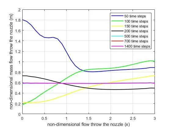
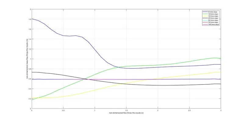
As you ca see in the graph that for each number of time steps how the flow is getting affected. At 50 time steps you can see it converge at a very slow rate, then at 1400 time steps you can see a straight line. this is what we needed to achieve. The above graph is of the non conservative code and the one below is the conservative code graph. they fairly show the same things happening.
CONSERVATIVE
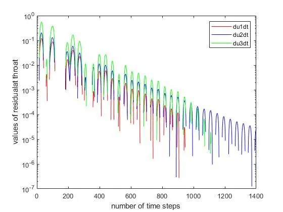
RESIDUAL VALUES AT THROAT FOR BOTH CONSERVATIVE AND NON CONSERVATIVE CODES ARE BELOW.
COMPARISON OF VARIOUS PARAMETERS WRT NOZZLE DISTANCE.
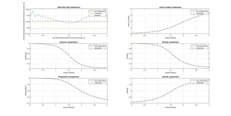
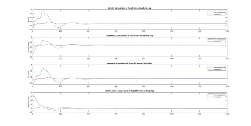
the graph below shows how the quantities behave through the nozzle. they are density, temperature, pressure and mach number respectively.
(blue: Non conservative.)