Week 6 - CHT Analysis on a Graphics card

Conjugate Heat Transfer simulation on A Graphics Card

Heat Transfer by Solids and Fluids

Heat Transfer in a Solid

In most cases, heat transfer in solids, if only due to conduction, is described by Fourier’s law defining the conductive heat flux, q, proportional to the temperature gradient: .

For a time-dependent problem, the temperature field in an immobile solid verifies the following form of the heat equation:

Heat Transfer in a Fluid

Due to the fluid motion, three contributions to the heat equation are included:

1. The transport of fluid implies energy transport too, which appears in the heat equation as the convective contribution. Depending on the thermal properties on the fluid and on the flow regime, either the convective or the conductive heat transfer can dominate.
2. The viscous effects of the fluid flow produce fluid heating. This term is often neglected, nevertheless, its contribution is noticeable for fast flow in viscous fluids.
3. As soon as a fluid density is temperature-dependent, a pressure work term contributes to the heat equation. This accounts for the well-known effect that, for example, compressing air produces heat.

Accounting for these contributions, in addition to conduction, results in the following transient heat equation for the temperature field in a fluid:

Conjugate Heat Transfer Applications

Effective Heat Transfer

Efficiently combining heat transfer in fluids and solids is the key to designing effective coolers, heaters, or heat exchangers.

The fluid usually plays the role of energy carrier on large distances. Forced convection is the most common way to achieve high heat transfer rate. In some applications, the performances are further improved by combining convection with phase change (for example liquid water to vapor phase change).

Here we are trying to simulate the heat transfer from a graphics card emanating heating from its processor, upon which other components like fins are attatched to increase the surface area and help in cooling.

So, we have an enclosure through which we pass air with various velocities. We dont have any exact values to validate the results. so what we do is that we observe if the total temperature in the enclosure is dropping with the change in velocity of the air. If that happens we can say our set up is correct.

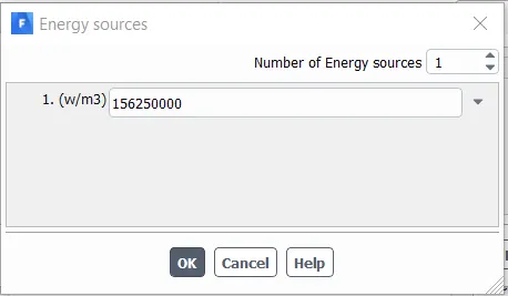
Here lets Assume 10 w of power is being supplied to the processor. Heat generated in `w/m^3` is given by divding the power with the volume of the conductor.

Volume of the conductor is 64e-009m^3. P/V = 156250000 `w/m^3`

Setup and results

1. Geometry

2. Meshing

3. Setup

4. results

1. GEOMETRY

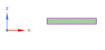
Processor

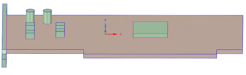
Base (with processor)

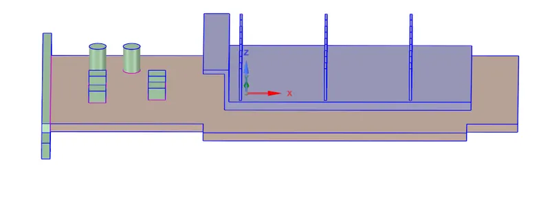
Final Graphic card assemble with aluminium fins

Materials used

Processor : titanium

Density = 4420 kg/m³

Base : Gold

Density = 19300 `(kg)/(m^3`

Fins = Aluminium

Density = 2700 `(kg)/m^3`

2. Meshing

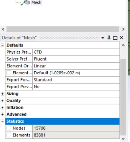
Initially we generate a base mesh and see if we have conformal mesh profile. For a conformal mesh we have to share topology in space claim. If we dont do that we cannot achieve conformal mesh and the solution wont be correct. After ensuring conformity, we move on to the setup. No methods have been used in meshing as this was the first experimental simulation to see if all the physics is correct.

In the above picture you can see that the no of elemets isnt that much. we have upto 500,000 elemets we can achieve for meshing with the student license.

3. Setup

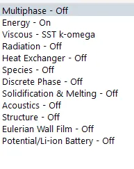
K-omega model used

energy is checked on for getting the temperature and ensuring air is at ambient temp at inlet.

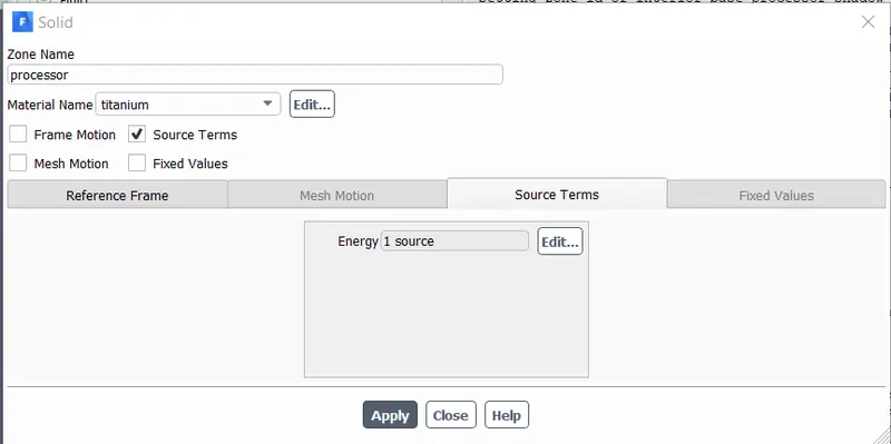
The boundary condition or heat generation origin is determined by us by using the cell zones and activating source terms. on doing so, we can input the amout of heat generated by the processor and how much of it is getting dissipiated. See below for the value of heat generated.

4. Results

Case 1

Here the velocity of inlet air is 1m/s

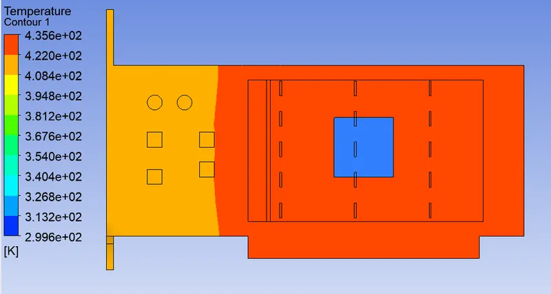
With the base mesh and air velocity, we have got a value of 435.6 K as the maximum temp.

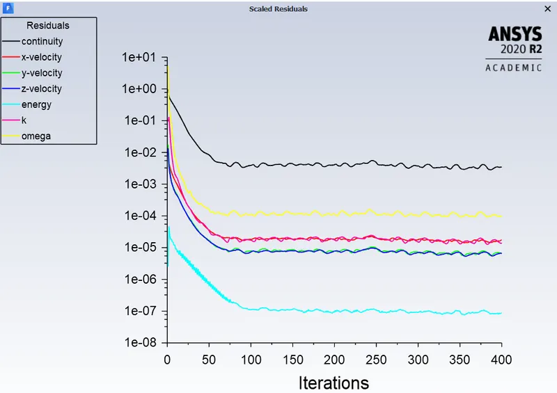
We can say that the solution has converged when the residual plot has a constant frequency like shown above after a point. As you can see after around 250 iterations the trend is constant and repetitive. The same goes for all the other cases.

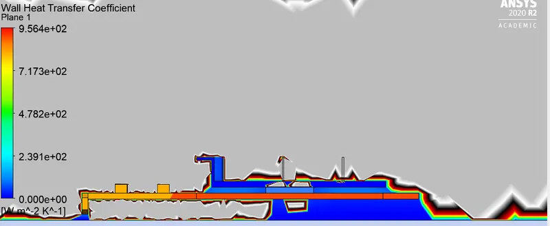
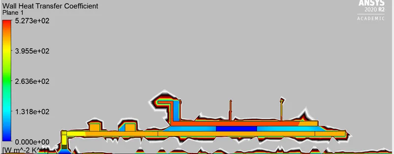
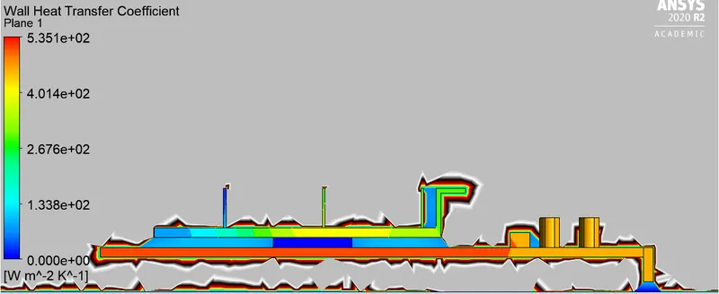
Wall heat transfer coefficient(coarse mesh)

(fine mesh) wall htc.

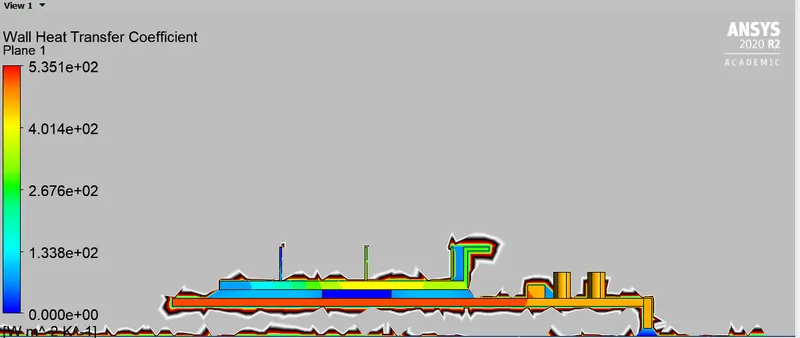
Notice how the HTC distribution is more accurate and even with finer mesh. This is in favour of the fact that better and finer mesh gives us a finer and accurate result.

Case 2

Refined mesh profile

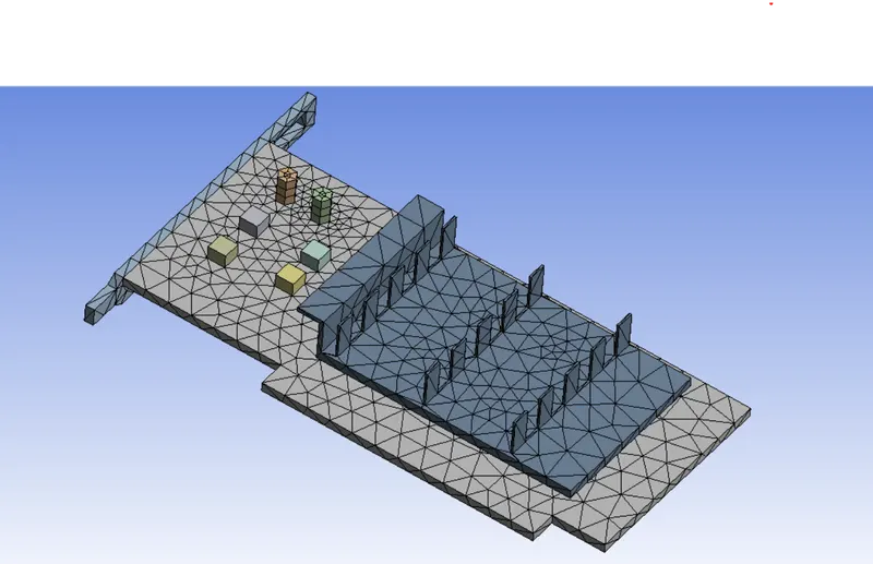
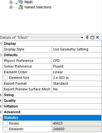
Here you can see the number of elements is above 200,000 which is is good compared to the base mesh. Here we get to capture the data and change in temperature better. After the refined mesh and for the same first case of velocity of air 1m/s, we got a max temp of 435.7K

velocity of inlet air is 3m/s

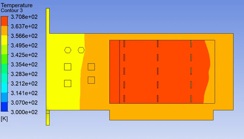
Max temp = 370.2K

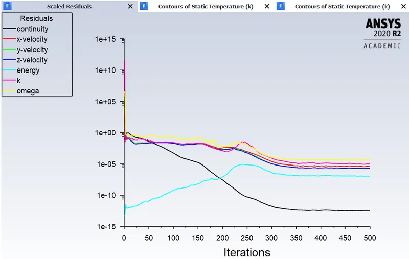
By looking at the residuals we can say that the solution has converged.

Case 3

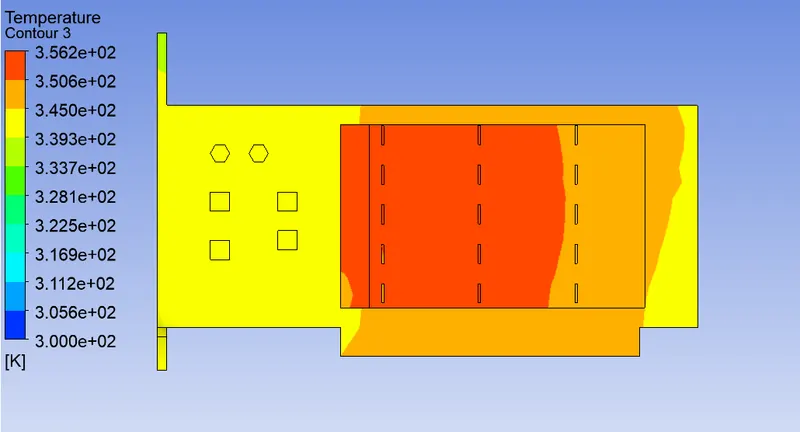
Max Temp = 356.2K

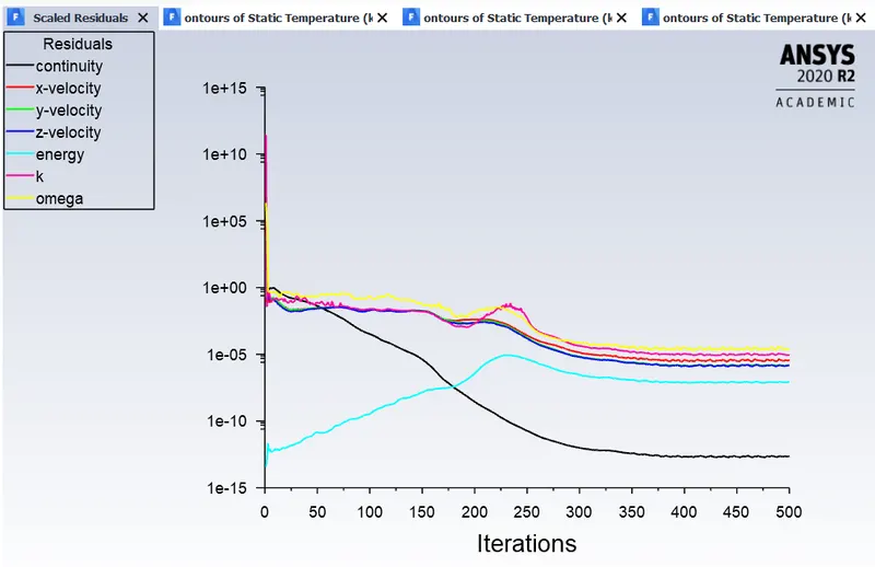
Here we can validate the results by noticing that as there is an increase in the velocity of inlet air, the temperature is decreasing. We can say that this simulation is technically sound.

Potential hotspots

from the Temp contour profiles we can say the main hot spots are the processor. From the processor heat is generated and then spread out to the aluminium fins. these fins help to spred out the heat that is generated and cool it faster. this is because the fins give extra surface area. Main hotspots being the processor and the fins.