Week 4 - CHT Analysis on Exhaust port
TITLE
Conjugate Heat Transfer analysis of an exhaust port.
OBJECTIVES
- Give a brief description of why and where a CHT analysis is used.
- Maintain the y+ value according to the turbulence model and justify the results.
- Calculate the wall/surface heat transfer coefficient on the internal solid surface & show the velocity & temperature contours in appropriate areas.
- How would you verify if the HTC predictions from the simulations are right? On what factors does the accuracy of the prediction depend on?
THEORY
Computational Fluid Dynamics(CFD) and more specifically conjugate heat transfer (CHT) analysis can accurately predict heat transfer by simultaneously solving all the relevant solid and flow field heat transfer processes, for example: conduction through solids, free and forced convection in the gases/fluids and thermal radiation.
The CHT approach has an advantage over FE Thermal Analyses in that wall heat transfer coefficients and their local variations on surfaces are directly calculated within the model rather than based on simplified empirical calculations. The CHT approach therefore has benefits for those applications where heat transfer is either non-uniform or difficult to calculate empirically.
Here we are conducting an analysis on the exhaust port of an engine. The Geometry of the exhaust port is in the image below. With this analysis
we can find out the Heat transfer coefficient.
The heat transfer coefficient or film coefficient, or film effectiveness, in thermodynamics and in mechanics is the proportionality constant between the heat flux and the thermodynamic driving force for the flow of heat (i.e., the temperature difference, ΔT):
The overall heat transfer rate for combined modes is usually expressed in terms of an overall conductance or heat transfer coefficient, U. In that case, the heat transfer rate is:

It is used in calculating the heat transfer, typically by convection or phase transition between a fluid and a solid. The heat transfer coefficient has SI units in watts per squared meter kelvin: W/(m2K).
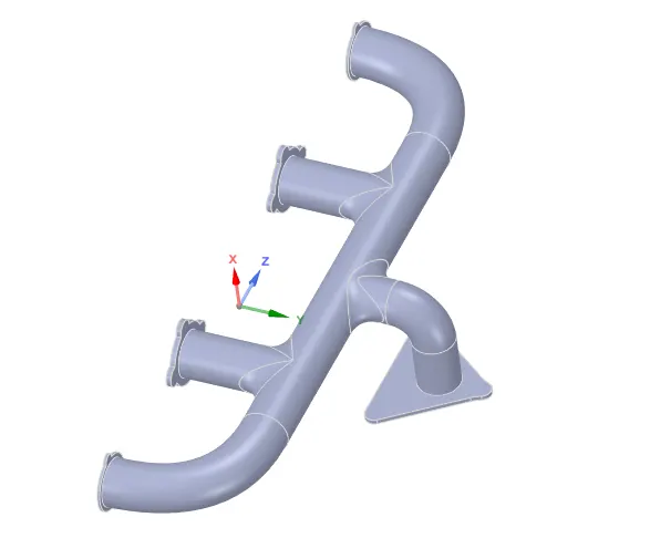 As you can see this exhaust port has 4 inlets and one outlet which then goes to the down pipe and then a catalytic converter,Which is followed by the end can.
So, What we are simulating is that hot air of 700K (approx. 420degree celcius) at a velocity of 5m/s. Then we get the value for the heat transfer coefficient.
We Use K-Epsilon model with scalable wall functions (default option in new version of Fluent). It will keep the Y+ above 11.06 so that it does not suffer the limitation of old standard wall functions.
hybrid wall function is applicable for all Y+ values. But keep in mind that these hybrid wall functions are designed for SA and K-Omega type models (SST included). However, K-Epsilon type models are designed for wall functions i.e. Y+ >30. But with one equation treatment for K-Epsilon models you can integrate them to viscous sub-layer. In this case K-Epsilon type models requires Y+<0.2. This is also known as enhanced wall treatment.
you can see that, strict value of Y+ < 2 for SST model and Y+ < 1 for SA model is now not must. So keeping Y+ upto 10 will give you same results as of mesh with Y+ ~ 1. Also note that for transition modeling (laminar to turbulence transition) you need mesh with Y+ < 1 everywhere along with the requirement of fine mesh in stream-wise direction.
Case 1
baseline mesh and no inflation layer.
Geometry
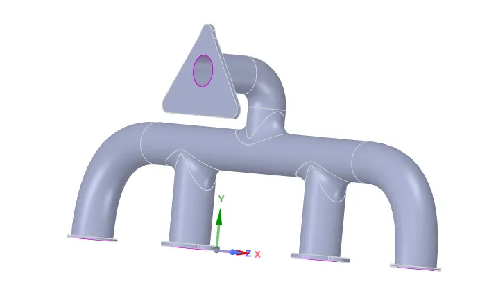
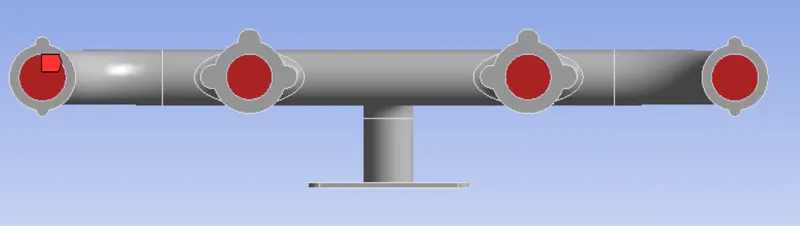
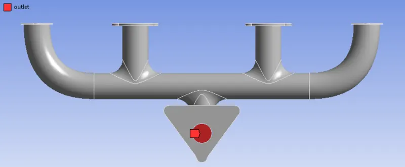
The above geometry represents an exhaust port with 4 inlets and 1 outlet. which are shown below. The idea is so simulate the flow of hot gasses(in this case air) and see how the temperature and the velocity vary. It is made of aluminium and passes hot air in this simulation.
BC For inflation layer
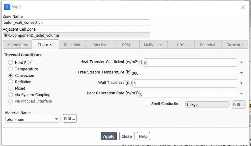
Heat transfer coefficient taken as 21.
INLET
OUTLET
Mesh (Baseline automatically generated)
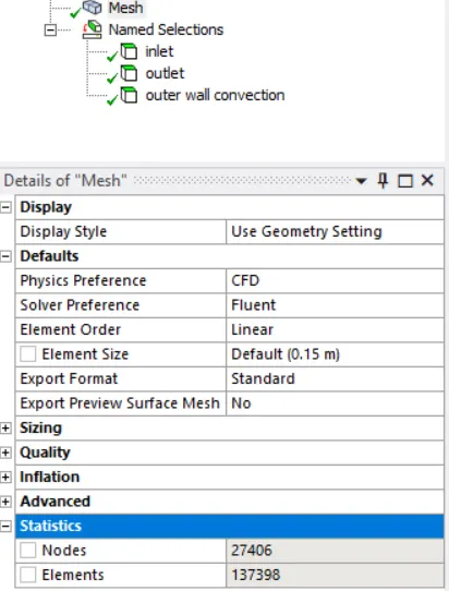
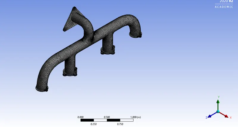
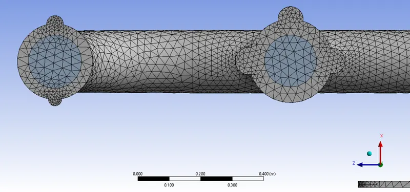
Conformal mesh achieved.
We are opting for conformal mesh to get good flux flow between the cells. If we dont achieve a conformal mesh the data we calculate will not be valid.
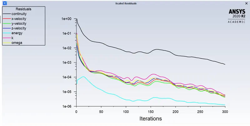
After running this simulation for 300 iterations we have the following results
RESULTS
Temperature contour.
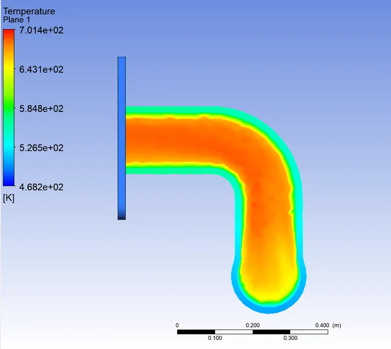
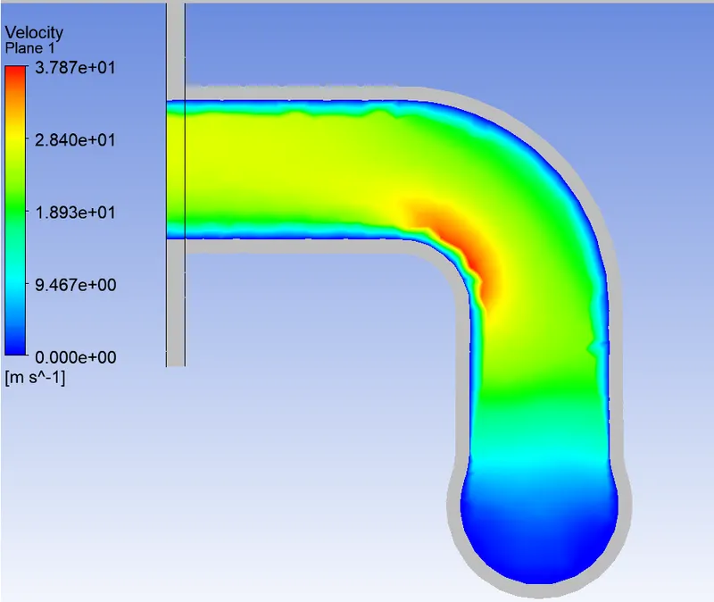
With this we can understand that the maximum heat will be generated at the bend of the outlet. This happens as all the inlets come and join to one flow. The law of conservation of mass helps us realize this and also, Velocity is the highest at the bend as well. The images of the same is below.
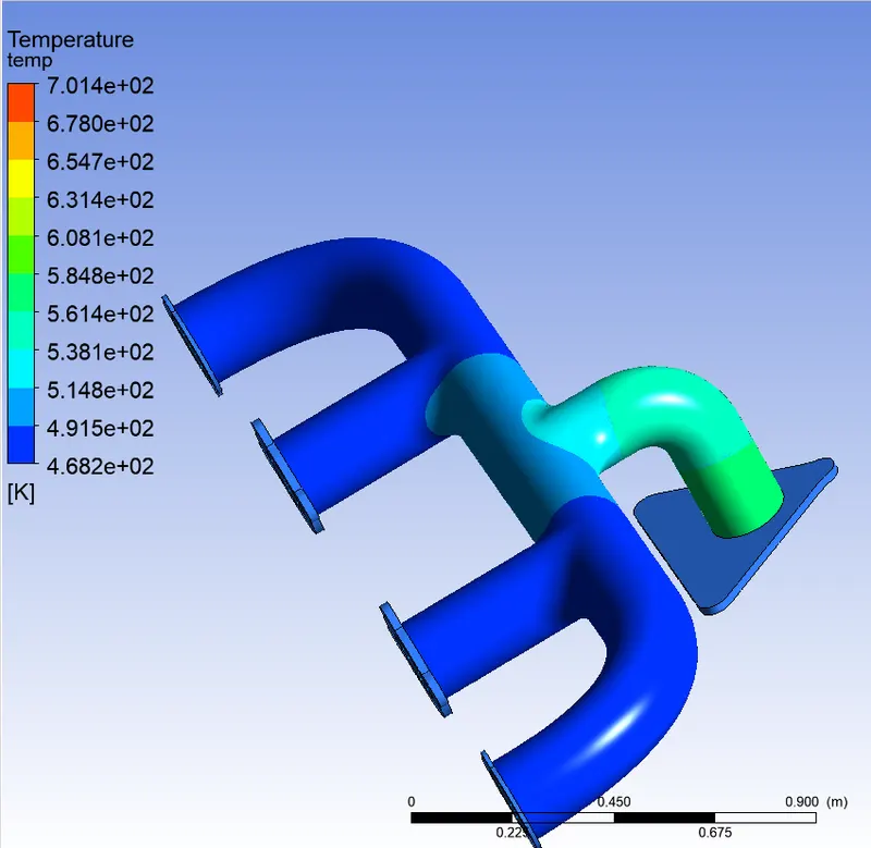
The below image shows the distribution of tempereature in the bend(outlet pipe) As ypu can see maximum heat is attained here.
Velocity contour
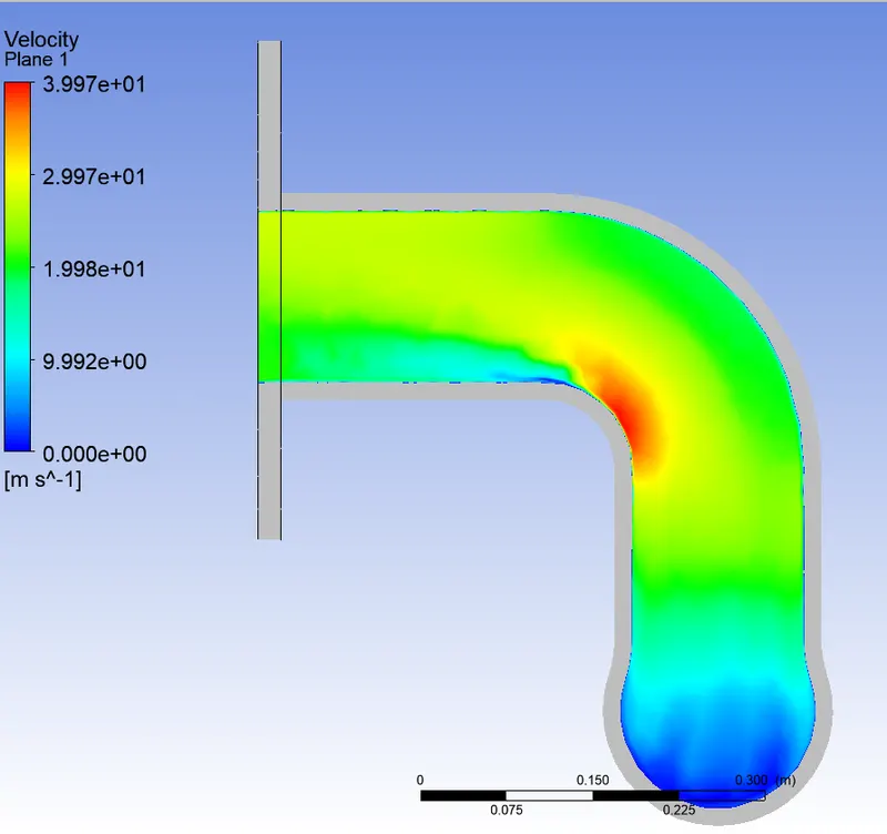
Here you can see the velocity contour at the bend. Notice the maximum velocity is at the bend shaded orange. This graphically proves that velocity is maximum where it should be and we have a good baseline mesh and setup to continue to our inflation casse results.
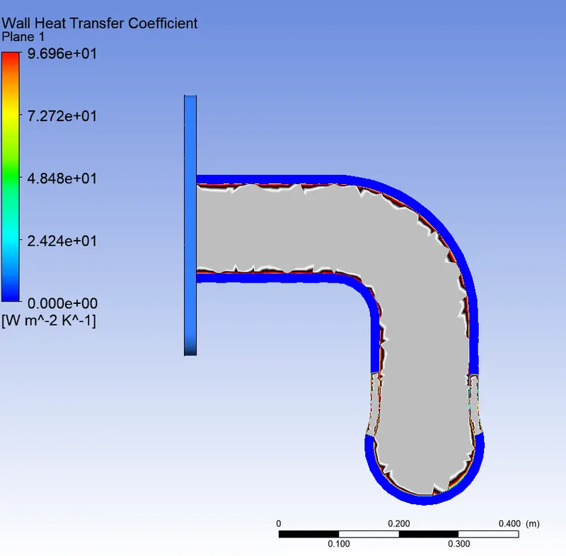
Wall Heat Transfer coefficient at the outlet pipe.
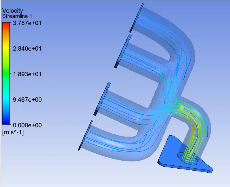
Streamlines
These stream lines show the flow of the gas(hot air) going from the inlet to the outlet. You can see where all the inlet flows mix. (Conservation of mass at play). And the velocity at the outlet will be maximum and as mentioned on top, velocity is maximum at the bend.
residuals
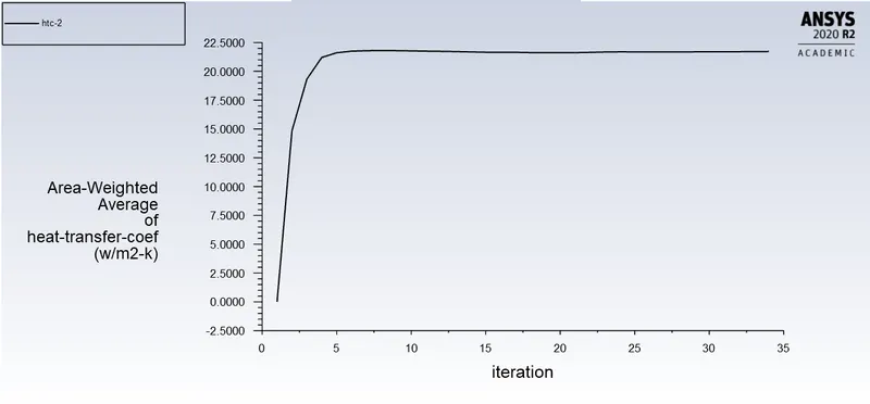
HTC(surface heat transfer)
Case 2 (mesh-refinement/inflation layer)
So, after we finish the simulation with the base mesh elements, now it is time to refine the mesh properties and run the simulation again with inflation layers.
All the boundary conditions remain the same. Here we create inflation layers of the fluid volume and name it accordingly. Once that is done we initialize the solution and add an xy-plot to get the wall y-plus chart.
So here we use the k-omega turbulance model to solve this solution as it is more suitable working with wall functions. Here what we should observe is that the physics should be defined in a better way.
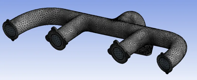
Mesh Details
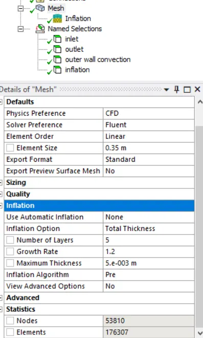
Mesh Profile
By looking at this mesh you can realize that this is much more finer and prescise which is goal here to capture more data.
Inflation layers
We add inflation layers to capture the physics more acuurately,Here we need the inflation layers only where there is interaction with the pipe walls. So we adopt total thickness method to add the inflation layers.
With maximum 5 layers and max thickness 5mm. This will help us be within the 5million cells range due to the license. 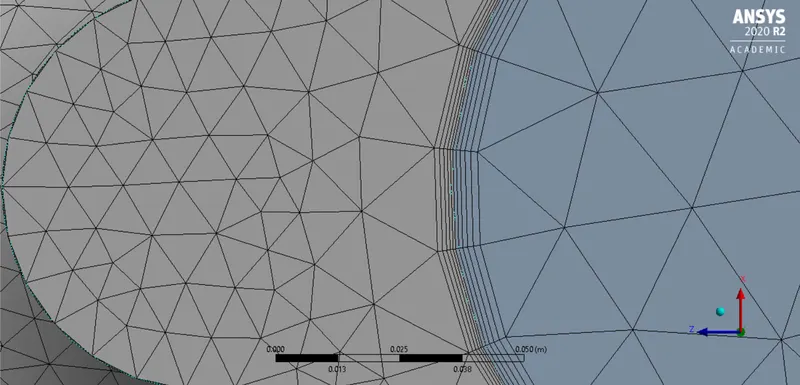
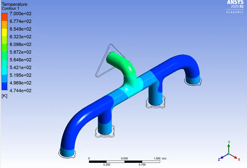
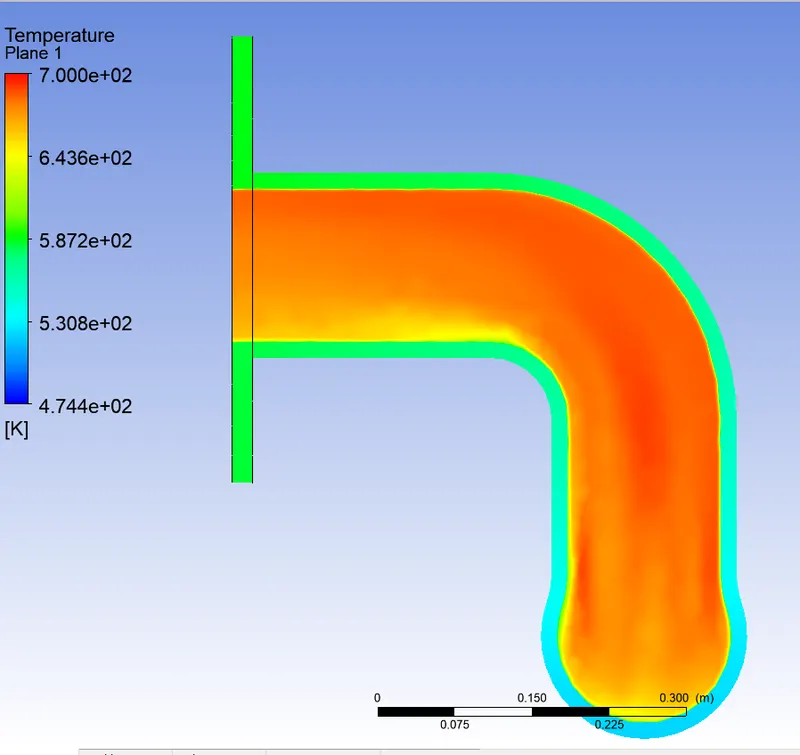
Temperature contour
Here you can see that the temperature profile is almost the same as the baseline mesh was also correct we are able to
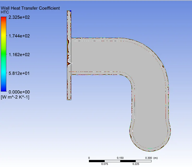
Wall Heat Transfer coefficient
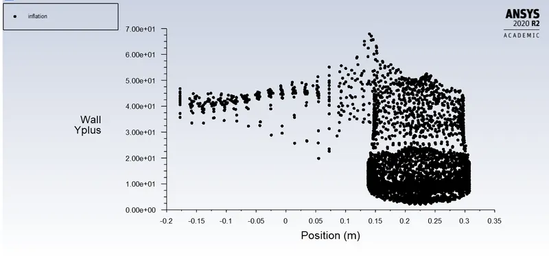
Below you can find the Y plus chart. As you can see that the majority of the inflation points lie within the range for k-omega (SST) turbulence model.(Y+<10)
The x-axis just shows us the position of the Geometry.
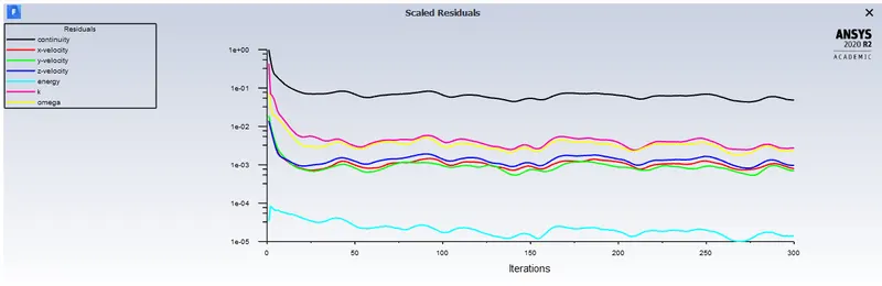
residuals
The Heat Transfer coefficient. Case 2.
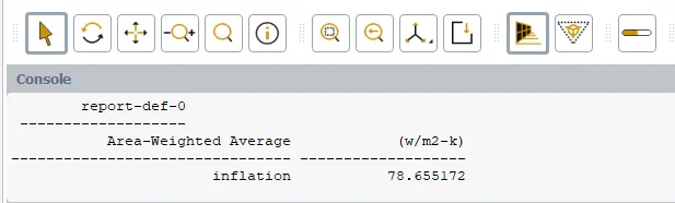
Here the wall heat transfer coefficient calculated is 78.655 `w/(m^2 K)`
Final Tabulation
| CASES | Nodes | Elements | HTC(`w/m^2 K`) |
| 1 | 137398 | 27406 | 21.720 |
| 2 | 176307 | 53810 | 78.655 |
Here as you can see that there is a marginal amount of difference between the two heat transfer coefficients of each case. So in the First case, it was just a baseline automated mesh generated by the computer, so that we can get the physics right before conducting the actual simulation.
Also, due to the Coarse nature of the mesh in case 1, in the beggining i used wall heat transfer coefficient to get the HTC for the fluid volume, had to create a separate named selection to achieve the same.
But i got a value which was not Valid (HTC = 3000000). So then i opted for Surface HTC which got me to the result mentioned above.
The surface heat transfer coefficient depends on the wall heat flux and the difference in temp of the wall and the reference temperature. Wall heat transfer coefficients depends on turbulence wall function quantities (like u* and T*).
 .
.