Week 4 - Genetic Algorithm

TITLE

Using the stalagmite mathematical model to check the Global maxima of a random,bounded and Known population space data, with the use of the Genetic algorithm.

EQUATIONS

STALAGMITE FUNCTION

`f(x,y)=f1,x f2,x f1,y f2,y`

`f1,x=[sin(5.1pi*x+0.5)]^6`

`f2,x=exp[-4ln(2)((x-0.0667)^2/0.64)]`

`f1,y=[sin(5.1pi*y+0.5)]^6`

`f1,y=[sin(5.1piy+0.5)]^6`

GENETIC ALGORITHM

A genetic algorithm (GA) is a method for solving both constrained and unconstrained optimization problems based on a natural selection process that mimics biological evolution. The algorithm repeatedly modifies a population of individual solutions. At each step, the genetic algorithm randomly selects individuals from the current population and uses them as parents to produce the children for the next generation. Over successive generations, the population "evolves" toward an optimal solution.

You can apply the genetic algorithm to solve problems that are not well suited for standard optimization algorithms, including problems in which the objective function is discontinuous, nondifferentiable, stochastic, or highly nonlinear.

Here we're using the ga() function for a data set of temperature versus the specific heat.

the syntax used in this code is as follows

x = ga(fun,nvars,A,b,Aeq,beq,lb,ub,nonlcon,intCon,options)

here

fun = function name

nvars = no of variables it accepts

A = Linear inequality constraints, specified as a real matrix. A is an M/nvars matrix, where M is the number of inequalities.

A encodes the M linear inequalities (ie: linear inequality contraints)

b = Linear inequality constraints, specified as a real vector.b is an M-element vector related to the A matrix. If you pass b as a row vector, solvers internally convert b to the column vector b(:).

b encodes the M linear inequalities

Aeq = Linear equality constraints, specified as a real matrix. Aeq is an Me/nvars matrix, where Me is the number of equalities.

Aeq encodes the Me linear equalities

beq = Linear equality constraints, specified as a real vector. beq is an Me-element vector related to the Aeg matrix. If you pass beq as a row vector, solvers internally convert beq to the column vector beq(:).

beq encodes the Me linear equalities

lb,ub = lower bounds(lb) and upper bounds(ub)

nonlcon = non linear constraints

intCon = to get our solution in an integer form

options = here it is used to specify the population.

CODE LOGIC

• We start off the code with clear all, close all and clc.
• We assign a set of data for x and y with the linspace() function.
• we assign a variable ' num_cases ' for the number of cases which helps us with this program.
• After creating a set of data for x and y we convert that into a 2D array [xx yy] using the meshgrid() function
• we begin the for loop in order to call in the stalagmite funtion which was defined.
• we used iteration variables i and j in the for loop .
• Now we move onto the first study with the genetic algorithm function with a radom set of variables which is taken by the ga() function and gives us the global maxima.
• we create an array variable for the return of the output from the ga() function which takes in the input from the stalagmite() function and has 2 variables.
• syntax for the ga() for study 1 is ga(@stalagmite,2)
• In figure(1) we plot the stalagmite mathematical model for the random variables using plot and use subplot function to plot the 2 graphs. This helps in creating a figure with 2 axes.
• We use the surf() function to plot the 3D surface plot with colors and grids.
• shading interp helps in varying the colors in one line segment
• plot3() function helps us to plot a 3D graph with each of the inputs it takes as a point of a vertex in each axes.
• we use the subplot command again to plot only the fopt or the random variables taken by the ga function.
• Notice that each time you run the trials for study 1 we get a different plot and set of variables. This is because of the ga() function.
• Moving on to the second study the cade is the same except with the ga() function. This is beacuse we use a different syntax to give the upper and lower bound constraints.
• This helps us get a better picture of where we get the global maxima.
• the syntax for the same is as follows ga(@stalagmite,2,[],[],[],[],[0;0],[1;1])
• with this we get a better plot of where the global maxima is.
• we also used the tic-toc command to get the time taken to compute and execute the code.
• Moving on to study 3, here we also define the population so that we get the most accurate results for the global maxima.
• slight change in the syntax of the ga() function. ga(@stalagmite,2,,[],[],[],[],[0;0],[1;1],[],[],options)
• options is the variable which hold the population number data.
• before calling the ga() function in the 3rd study we use optimoptions() to get the most optimum data.
• we use the same variable for defining the population space the ga() function to consider.
• plotting the same gives us the most accurate position and points of the global maxima.

CODE

Code for stalagmite function with 3 different studies.

clear all
close all
clc

x = linspace(0,0.6,150);
y = linspace(0,0.6,150);
num_cases = 50;
[xx yy] = meshgrid(x,y);
 % Evaluating the stalagmite function
 for i = 1:length(xx)
     for j = 1:length(yy)
         input_vector(1) = xx(i,j);
         input_vector(2) = yy(i,j);
         f(i,j) = stalagmite(input_vector);
     end
 end


% study 1 with radom search space 
for i = 1:num_cases
    [inputs, fopt(i)] =  ga(@stalagmite, 2);
    xopt(i) = inputs(1);
    yopt(i) = inputs(2);
    
end


figure(1)
subplot(2,1,1)
hold on
surfc(x,y,-f)
shading interp
plot3(xopt,yopt,-fopt,'marker','o','markersize',5,'markerfacecolor','r')
title('unbounded inputs')
subplot(2,1,2)
plot(-fopt)
xlabel('iterations')
ylabel('function minimum')


tic
%study 2 with upper and lower bounds

for i = 1:num_cases
    [inputs, fopt(i)] = ga(@stalagmite,2,[],[],[],[],[0;0],[1;1]);
    xopt(i) = inputs(1);
    yopt(i) = inputs(2);
end
study2_time = toc

figure(2)
subplot(2,1,1)
hold on
surfc(x,y,-f)
shading interp
plot3(xopt,yopt,-fopt,'marker','o','markersize',5,'markerfacecolor','r')
title('bounded inputs')
subplot(2,1,2)
plot(-fopt)
xlabel('iterations')
ylabel('function minimum')
ylim([0 2])


% Study 3 with bounds and population size
options = optimoptions('ga');
options = optimoptions(options,'populationsize',250);


tic

for i = 1:num_cases
    [inputs, fopt(i)] = ga(@stalagmite,2,[],[],[],[],[0;0],[1;1],[],[],options);
    xopt(i) = inputs(1);
    yopt(i) = inputs(2);
end
study3_time = toc

figure(3)
subplot(2,1,1)
hold on
surfc(x,y,-f)
shading interp
plot3(xopt,yopt,-fopt,'marker','o','markersize',5,'markerfacecolor','r')
title('bounded inputs')
subplot(2,1,2)
plot(-fopt)
xlabel('iterations')
ylabel('function minimum')
ylim([0 2])

RESULTS

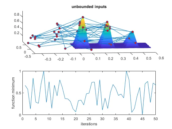
The above image shows how the global maxima varies with a random population sample.

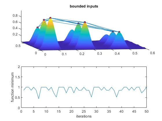
This image shows how the global maxima varies when you have specified upper and lower bounds.

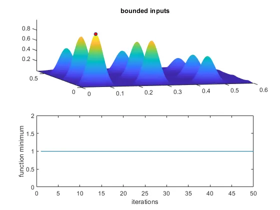
This image shows how the global maxima is accurately found through calculations with specified upper and lower bounds, and a population size of 400.

ERRORS

This is the error i got when i had left out to use a bracket at the end of a function.