Week 3 - Taylor table method and Matlab code

TITLE

Derivation of the 4th order approximations of the second order derivatives.

OBJECTIVE

To write a code in matlab which uses the taylor series approximation equations to get the plot of 3 types of approximations and compare them and understand which gives us the best approximations with the least error possible.

EQUATIONS USED

Here the main equation used is the taylor series expansion series. We have taken a function `f(x) = (e^x)*cos(x)`

The taylor series expansion in general form is given below

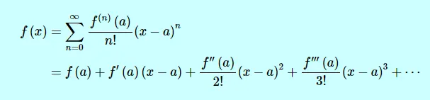
Now we calculate and find the value of the given function at different points usuing the taylor series table and approximations. The central difference approximation will take even number of points of the number of nodes -calculated in the equation shown below- on either side of  where the function f(x) lies. This is graphically represented below. Then when we move on to right and left skewed approximations we take the points either to the right or the left of where the function f(x) lies. Each of the said approximations is graphically represented below in the order 1,2 and 3.

Order of accuracy  = No. of nodes in the stencil- Order of the derivative+1 [This is for central approximations]

Order of accuracy  = No. of nodes in the stencil- Order of the derivative [This is for skewed approximations]

 

1. Central Approximation

         (i-2)      (i-1)         (i)       (i+1)       (i+2) 

______^______^______^______^______^______

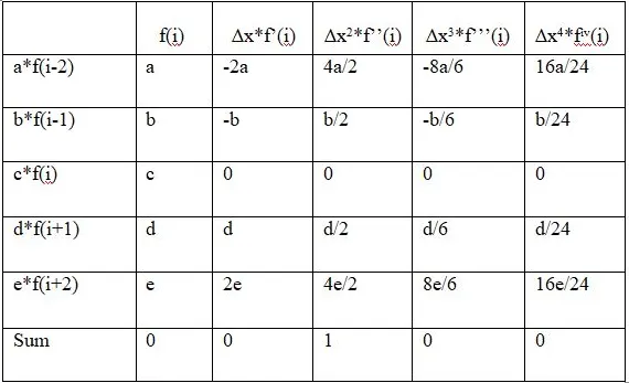
Hypothesis Equation

proof of accuracy  = 5 (nodes)- 2 (order of derivative)+1 = 4.

2. Right Skew Approximation

          (i)         (i+1)     (i+2)     (i+3)      (i+4)      (i+5)      

______^______^______^______^______^______^______

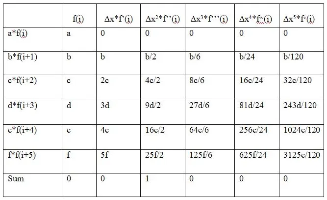
Hypothesis Equation

proof of accuracy  = 6 (nodes)- 2 (order of derivative) = 4.

3. Left Skew Approximation

         (i-5)       (i-4)       (i-3)      (i-2)       (i-1)        (i)

______^______^______^______^______^______^______

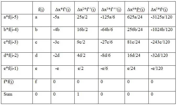
Hypothesis Equation

proof of accuracy  = 6 (nodes)- 2 (order of derivative) = 4.

The taylor table that you see above are nothing but the taylor series expansions of the function f(x) at each points of the approximations taken respectively.

CODE LOGIC

• We start the code with clear all, close all and clc.
• Initialize x and dx.
• For loop for accessing each of the functions and recieving all the necessary data step wise.
• plotting all the required graphs
• using lengend and labels to name the graph and make it look informative.
• Moving on to the function definitions, as you can see in the above tables , all those values can be taken as simultaneous of each part and solved for all the coefficients a,b,c,d,e and in some cases f.
• so we find the coefficients of the same using matrices.
• before that we input the second order derivative of the given derivative.
• We perfom a simple  `X = A^-1*B`
• where all the coefficients we need will be stored in the matrix X
• we assign variable names for each of the data in the column vector X
• This will help us write the hypothesis equation with ease.
• After that we calculate the error and we send it back to the main function to help us plot the graph of each approximations and their errors.
• This continues for both the other function which is given below.

CODE

% Taylor table code

clear all
close all
clc
  % Initialisation  
x = pi/3;
dx = linspace(pi/3,pi/3000,200);
for i = 1:length(dx)
    central_diff(i) = central_difference(x,dx(i));
    right_skew(i) = right_skw(x,dx(i));
    left_skew(i) = left_skw(x,dx(i));
end
 %plotting all the graphs
 figure(1)

 loglog(dx,central_diff,'linewidth',1,'color','r')
 hold on
 loglog(dx,right_skew,'linewidth',2,'color','g')
 hold on
 loglog(dx,left_skew,'linewidth',3,'color','b')
 xlabel('dx')
 ylabel('Errors')
 legend('Central differencing error','Right skewed error','Left skewed error');
 axis([(10^-3) (10^0) (10^-10) (10^8)])
 
 

All the function definitions

%function definition for central differencing

function central_error =  central_difference(x,dx)
% Function  f(x) = exp(x)*cos(x)
    second_order_deriv = -2*(exp(x))*sin(x);
    
    % Matrix calculated data for each of the coefficients
   A = [1 1 1 1 1;-2 -1 0 1 2;2 0.5 0 0.5 2;-8/6 -1/6 0 1/6 8/6;16/24 1/24 0 1/24 16/24];
B = [0;0;1;0;0];

X = inv(A)*B;

a = X(1);
b = X(2);
c = X(3);
d = X(4);
e = X(5);
%Central difference calculation
    
      central_difference = ((a*(exp(x-(2*dx))*(cos(x-(2*dx))))) + (b*(exp(x-(1*dx))*(cos(x-(1*dx))))) + (c*(exp(x))*(cos(x))) +(d*(exp(x+(1*dx))*(cos(x+(1*dx))))) + (e*(exp(x+(2*dx))*(cos(x+(2*dx))))))/(dx^2);

% Error
central_error = abs(second_order_deriv-central_difference)
end

% Skewed right function
function Rskew_error = right_skw(x,dx)

% Function  f(x) = exp(x)*cos(x)
    second_order_deriv = -2*(exp(x))*sin(x);


    % Matrix calculated data for each of the coefficients
A = [1 1 1 1 1 1;0 1 2 3 4 5;0 0.5 2 9/2 16/2 25/2;0 1/6 8/6 27/6 64/6 125/6;0 1/24 2/3 81/24 256/24 625/24;0 1/120 32/120 243/120 1024/120 3125/120];
B = [0;0;1;0;0;0];
X =inv(A)*B;
a = X(1);
b = X(2);
c = X(3);
d = X(4);
e = X(5);
f = X(6);




% Right skew calculation
right_skw = ((a*exp(x)*cos(x)) + (b*exp(x+dx)*cos(x+dx)) + (c*exp(x+(2*dx))*cos(x+(2*dx))) +(d*exp(x+(3*dx))*cos(x+(3*dx))) + (e*exp(x+(4*dx))*cos(x+(4*dx))) + (f*exp(x+(5*dx))*cos(x+(5*dx))))/(dx^2);


% Error
Rskew_error = abs(second_order_deriv-right_skw)
end

% Skewed left function
function Lskew_error = left_skw(x,dx)

% Function  f(x) = exp(x)*cos(x)
    second_order_deriv = -2*(exp(x))*sin(x);

% Matrix calculated data for each of the coefficients
A = [1 1 1 1 1 1;-5 -4 -3 -2 -1 0;25/2 16/2 9/2 4/2 1/2 0;-125/6 -64/6 -27/6 -8/6 -1/6 0;625/24 256/24 81/24 16/24 1/24 0;-3125/120 -1024/120 -243/120 -32/120 -1/120 0];
B = [0;0;1;0;0;0];
X = inv(A)*B
a = X(1);
b = X(2);
c = X(3);
d = X(4);
e = X(5);
f = X(6);

% Right skew calculation
left_skw = ((a*exp(x-(5*dx))*cos(x-(5*dx))) + (b*exp(x-(4*dx))*(cos(x-(4*dx)))) + (c*exp(x-(3*dx))*cos(x-(3*dx))) +(d*exp(x-(2*dx))*cos(x-(2*dx))) + (e*exp(x-dx)*cos(x-dx))+(f*exp(x)*cos(x)))/(dx^2);

% Error
Lskew_error = abs(second_order_deriv-left_skw)
end

RESULTS 

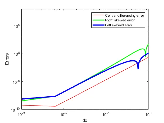
As you can see in the results graph that central approximation method yeilded a better approximation with  the least amount of error.

ERRORS FACED

The main errors i faced was i was getting completely wrong graph of each of the approximations. this was because the number of parenthesis was un-even in my equations in the function definition part.

To avoid this was why i used the letter of the alphabet to store the matrix data and could easily access them at the defition of the equation for each approximation.