Week 5 - Mid term project - Solving the steady and unsteady 2D heat conduction problem
TITLE
Solving the 2D steady and unsteady state conditions of the heat conduction equation.
EQUATIONS USED
The 2D heat equation is

At steady state we have equation
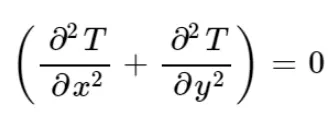
the above equation is transformed into a numerical form with the central differencing scheme.
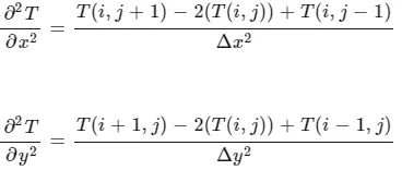

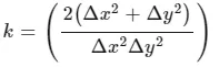
Where
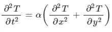
The transient state equation is

For transient implicit method
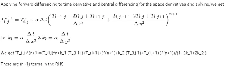
The above shown equations are solved using jacobi, gauss sieldel and succesive over relaxation methods and/or implicit time marching method.
CODE LOGIC
- First we start off with the clear all, close all and clc commands.
- Then we need the inputs
- nx and ny will act as our spacial loop variables.
- dx is the space between consecutive points in the 'x' array which we crerated with the linspace command.
- dy is is the same for array 'y'.
- Next we include the 3 methods of iterative solvers.
- It has been made into a menu with the input being the type of method to be used to solve the equation.
- w will be the variable responsible for the determination of the method used to solve the equation.
- After you type in the method to be used and press enter it will execute that method and provide you with the results.
- Then we make our temperature array so that we get to access all the data in it.
- we define the tolerance and error.The program should run based on the characteristic of the error and its relativity with the tolerence.
- the condition would be that if the error is greater than the tolerence then the code should run.
- we use 2 for loops for us to navigate throught the space loop.
- then we do the necessary calculations and update the array we go on.
- Updating the array(Temperature array) is important because we need those values for executing the program.
- We do the same for all the 3 methods
- Finally we plot our results.
CODE(STEADY STATE EXPLICIT)
% 2D Heat conduction steady state explicit

clear all
close all
clc

% INITIALISATION
nx = 100;
ny = 100;
x  =  linspace(0,1,nx);
dx = x(2)-x(1);
y  = linspace(0,1,ny);
dy = y(2)-y(1);


% USER DEFINED METHODS
% 1. JACOBI
% 2. GS
% 3. SOR
fprintf('Enter the number of the method to be used   n')
fprintf('1. JACOBI n 2. GS n 3. SOR n')
w = input('choose 1, 2 or 3 : ')


% GIVEN TEMPS

T = 300*ones(ny,nx);

T(:,1)  = 400;
T(1,:)  = 600;
T(:,end)= 800;
T(end,:)= 900;

Told = T;

K = (2*(dx^2+dy^2))/(dx^2*dy^2);

tol   = 1e-4;
error = 9e9;


% ITERATION 1 (it_1) JACOBI
it_m = w;

if w == 1

    tic
    iter = 0;
    while(error > tol)

        for i = 2:nx-1

            for j = 2:ny-1
               term_1 = (Told(i-1,j)+Told(i+1,j))/dx^2;
    term_2 = (Told(i,j-1)+Told(i,j+1))/dy^2;

                T(i,j) = ((1/K)*term_1) +((1/K)*term_2);
            end
        end
        error =max( max(abs(Told-T)))
        Told = T;
        iter = iter+1;
    end
%     iter = iter+1;
    time = toc


% ITERATION 2 (it_1) GAUSS SIEDEL

elseif w == 2

    tic
    iter = 0;
    while(error > tol)

        for i = 2:nx-1

            for j = 2:ny-1
               term_1 = (T(i-1,j)+Told(i+1,j))/dx^2;
    term_2 = (T(i,j-1)+Told(i,j+1))/dy^2;

                T(i,j) = ((1/K)*term_1) +((1/K)*term_2);
            end
        end
        error = max(max(abs(Told-T)))
        Told = T;
        iter = iter+1;
    end
%     iter = iter+1;
    time = toc


elseif w == 3
    omg = 1.8;
     tic
    iter = 0;
    while(error > tol)

        for i = 2:nx-1

            for j = 2:ny-1
               term_1 = (T(i-1,j)+Told(i+1,j))/dx^2;
    term_2 = (T(i,j-1)+Told(i,j+1))/dy^2;

                T(i,j) = ((1/K)*term_1) +((1/K)*term_2);
                T(i,j) = Told(i,j)*(1-omg)+(omg*T(i,j));
            end
        end
        error = max(max(abs(Told-T)))
        Told = T;
        iter = iter+1;
    end
%     iter = iter+1;
    time = toc
end

% plotting

[c,h] = contourf(x,y,T)
clabel(c,h)
colorbar
colormap(jet)
ax = gca;
ax.YDir = 'reverse';
xlabel('x axis')
ylabel('y axis')
title({'steady statet temp profile';['iteration method =',num2str(it_m)];['Number of iterations =',num2str(iter)];['simulation time = ',num2str(time)]})
grid on
RESULTS
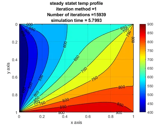
JACOBI METHOD
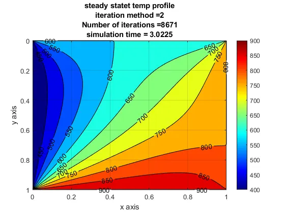
GAUSS SIEDEL METHOD
SOR METHOD
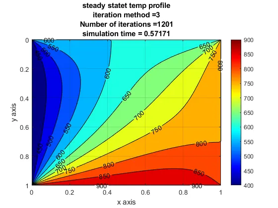
Above shown images are the plots for the same equation with the different methods used to solve them. namely Jacobi, Gauss Siedel and SOR. as you ca see that the number of iterations in each case is different. if it wasnt different then it would defeat the purpose of this program. the no of iteration decrease as the method changes cosecutively in the same order.
we can say that SOR method got to the solution with much less effort than the other 2 methods and it took a shorter time achieving the same. This is what is beneficial for any company. you get the to the solution with the least no of iterations and most accuracy.
CODE(TRANSIENT EXPLICIT)
% TRANSIENT STATE HEAT CONDUCTION EQUATION
% EXPLICIT METHOD

clear all
close all
clc

% INITIALISATION

nx = 100;
ny = nx;
 dt = 0.14;
t = 2000;
nt = 8000;
alpha = 1.75e-4;

x = linspace(0,1,nx);
dx = x(2)-x(1);
y = linspace(0,1,ny);
dy = y(2)-y(1);
CFL = alpha*dt*((1/dx^2)+(1/dy^2));


%TEMP MATRIX

T = 300*ones(ny,nx);

T(:,1)  = 400;
T(1,:)  = 600;
T(:,end)= 800;
T(end,:)= 900;

Told = T;

K1 = alpha*dt/dx^2;
K2 = alpha*dt/dy^2;


itr = 0;
tic


% TIME LOOP

for k = 1:nt

    for j = 2:ny-1

        for i = 2:nx-1

            H      = (Told(i-1,j) -(2*Told(i,j)) +Told(i+1,j));
            V      = (Told(i,j-1) -(2*Told(i,j)) + Told(i,j+1));
            T(i,j) =  Told(i,j)+ (H*K1) + (V*K2);
        end
    end
    Told = T;
    itr = itr +1;

end
time = toc;


% plotting

[c,h] = contourf(x,y,T)
clabel(c,h)
colorbar
colormap(jet)
ax = gca;
ax.YDir = 'reverse';
xlabel('x axis')
ylabel('y axis')
title({'steady state temp profile';['Number of iterations =',num2str(itr)];['simulation time = ',num2str(time)]})
grid on
RESULTS
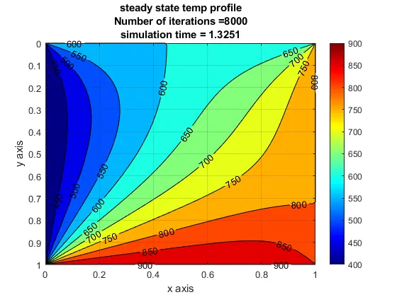
Here in the transient state we did not need a condition to be fulfilled in order to carry on the calculation which makes it easier to get to the solution. So here unlike in the steady state program we dont need a while loop.
When you compare that with the number of iterations in the steady state, theres not much of a difference. So here we also used a time marching technique to get to the solution.the for loops are for the time step iterating to the next time steps and futher on. at t = 1000 seconds, the solution seems to be steady.
CODE(TRANSIENT IMPLICIT)
% TRANSIENT STATE HEAT CONDUCTION EQUATION
% IMPLICIT METHOD


clear all
close all
clc


% INITIALISATION

nx = 50;
ny = nx;
dt = 10;
t = 1000;
nt = t/dt;
alpha = 1.75e-4;

x = linspace(0,1,nx);
dx = x(2)-x(1);
y = linspace(0,1,ny);
dy = y(2)-y(1);
CFL = alpha*dt*((1/dx^2)+(1/dy^2));


%TEMP MATRIX

T = 300*ones(ny,nx);

T(:,1)  = 400;
T(1,:)  = 600;
T(:,end)= 800;
T(end,:)= 900;

Told = T;
Tp = T;

K1 = alpha*dt/dx^2;
K2 = alpha*dt/dy^2;

tol   = 1e-4;


% USER DEFINED METHODS
% 1. JACOBI
% 2. GS
% 3. SOR
fprintf('Enter the number of the method to be used   n')
fprintf('1. JACOBI n 2. GS n 3. SOR n')
w = input('choose 1, 2 or 3 : ')

if w == 1
fprintf(' JACOBI METHOD n')            % JACOBI

    tic
    iter = 1;
    for k = 1:nt

            error = 1;
        while( error > tol )

        for j = 2:ny-1

            for i = 2:nx-1

                t1 = (1/(1+(2*K1)+(2*K2)));
                t2 = K1*t1;
                t3 = K2*t1;

                H = Told(i-1,j)+Told(i+1,j);
                V = Told(i,j-1)+Told(i,j+1);
           T(i,j) = (Tp(i,j)*t1)+(H*t2)+(V*t3);
            end
        end
        error = max(max(abs(T-Told)));
        Told = T;
        iter = iter+1;
        end
        Tp = T;
    end
    time = toc;


    % GS METHOD


elseif w == 2      % GS
    fprintf(' GS METHOD n')
    tic
    iter = 1;
    for k = 1:nt

            error = 1;

        while( error > tol )


        for j = 2:ny-1

            for i = 2:nx-1

                t1 = (1/(1+(2*K1)+(2*K2)));
                t2 = K1*t1;
                t3 = K2*t1;

                H = T(i-1,j)+Told(i+1,j);
                V = T(i,j-1)+Told(i,j+1);
           T(i,j) = (Tp(i,j)*t1)+(H*t2)+(V*t3);
            end
        end
        error = max(max(abs(T-Told)));
        Told = T;
        iter = iter+1;
        end
        Tp = T;
    end
    time = toc;


    % SOR METHOD


elseif w == 3
    fprintf(' SOR METHOD n')    % SOR
omega = 1.4;
    tic
    iter = 1;
    for k = 1:nt

            error = 1;

        while( error > tol )

        for j = 2:ny-1

            for i = 2:nx-1

                t1 = (1/(1+(2*K1)+(2*K2)));
                t2 = K1*t1;
                t3 = K2*t1;

                H = T(i-1,j)+Told(i+1,j);
                V = T(i,j-1)+Told(i,j+1);
           T(i,j) = (Tp(i,j)*t1)+(H*t2)+(V*t3);
           T(i,j) = Told(i,j)*(1-omega)+omega*T(i,j);
            end
        end
        error = max(max(abs(T-Told)));
        Told = T;
        iter = iter+1;
        end
        Tp = T;
    end
    time = toc;
end


[c,h] = contourf(x,y,T)
clabel(c,h)
colorbar
colormap(jet)
ax = gca;
ax.YDir = 'reverse';
xlabel('x axis')
ylabel('y axis')
title({'steady state temp profile';['iteration method =',num2str(w)];['Number of iterations =',num2str(iter)];['simulation time = ',num2str(time)]})
RESULTS
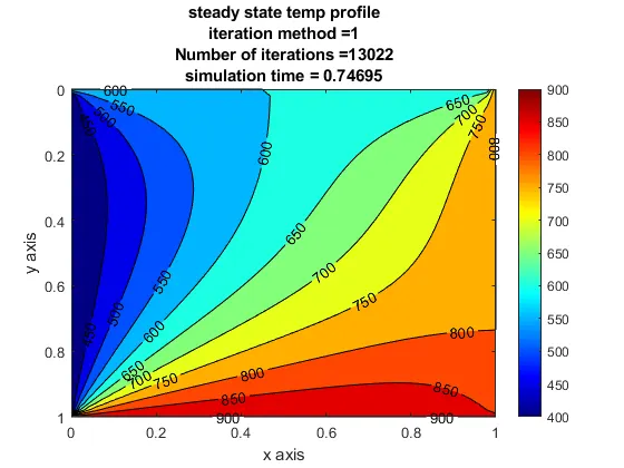
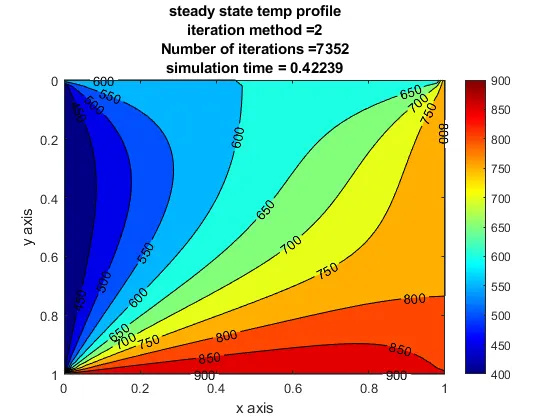
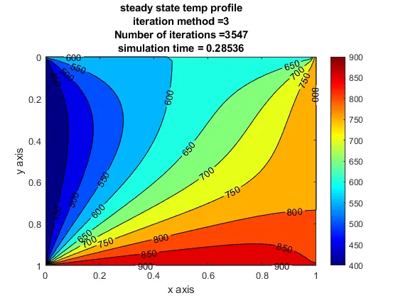
These are the results from which we solved the transient equation with iterative solvers. The same 3, jacobian, gs and sor. the same trend applies here as well, the least no of iterations is in the sor method rather than the other two. As you can see all the graphs are almost exactly the same. but the way the solution was attained was different and the amount of time and effort taken by the program to execute the same was different.
The coding in this section was almost as similar to the steady state method albeit a few changes in the equation