Project 2 - Rankine cycle Simulator
TITLE
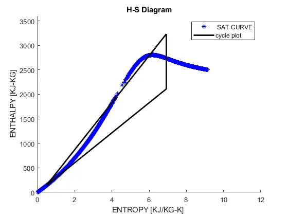
To write a code to simulate a rankine cycle and shows its T-S(TEMP-ENTROPY) and H-S(ENTHALPY-ENTROPY) diagrams.
THEORY
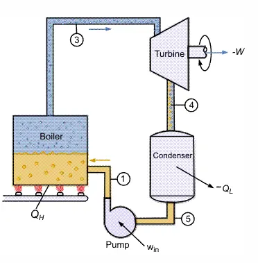
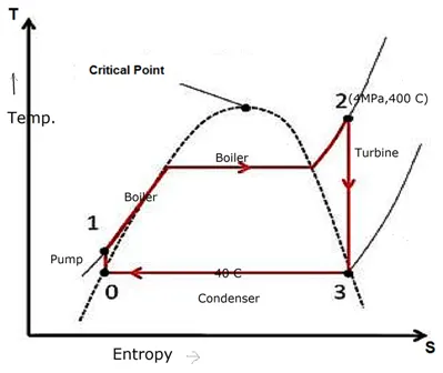
Below figures give you a breif idea of how a rankine cycle works and how the T-S diagram Aand H-S should look like.
S -->
[KJ/KG-K].
1-2-3 Isobaric Heat Transfer. High pressure liquid enters the boiler from the feed pump (1) and is heated to the saturation temperature (2). Further addition of energy causes evaporation of the liquid until it is fully converted to saturated steam (3).
3-4 Isentropic Expansion. The vapor is expanded in the turbine, thus producing work which may be converted to electricity. In practice, the expansion is limited by the temperature of the cooling medium and by the erosion of the turbine blades by liquid entrainment in the vapor stream as the process moves further into the two-phase region. Exit vapor qualities should be greater than 90%.
4-5 Isobaric Heat Rejection. The vapor-liquid mixture leaving the turbine (4) is condensed at low pressure, usually in a surface condenser using cooling water. In well designed and maintained condensers, the pressure of the vapor is well below atmospheric pressure, approaching the saturation pressure of the operating fluid at the cooling water temperature.
5-1 Isentropic Compression. The pressure of the condensate is raised in the feed pump. Because of the low specific volume of liquids, the pump work is relatively small and often neglected in thermodynamic calculations.
Since we do not know the exact vapor quality of the outlet steam, we have to determine this parameter. State 4 is fixed by the pressure p4.
The enthalpy for the state 3 can be picked directly from steam tables, whereas the enthalpy for the state 4 must be calculated using vapor quality.
Enthalpy for state 1 can be picked directly from steam tables.
State 2 is fixed by the pressure p2, and the specific entropy is constant for the isentropic compression.
Also note that the points on the saturation curve dont necessarily have equations for calculations, it can either be be in the steam table or we get it through the state points being equal.
NOTE : THE NOTATIONS USED IN THE IMAGE ARE NOT SAME AS THOSE USED IN THE EQUATIONS
EQUATIONS USED
Turbine Work
`W_t = H1-H2`
Pump Work
`W_P = H4-H3`
Heat Addition
`Q_"in" = H1-H4`
Heat Rejection
`Q_(out) = H2-H3`
Net work done
`W_("net") = W_t-W_p`
Thermal Efficiency
`"therm_eff" = (W_("net")/Q_("in"))*100`
Specific steam consumption
`"SSC" = 3600/W_("net")`
Back Work Ratio
`"BW_R" = W_p/W_t`
CODE LOGIC
- We start off the code with the basic clear functions. clear all,close all and ccl.
- Now to input the values that we need in real time we use a slightly different approach in writing this code.
- Initially we use the fprintf() command to display whatever it is that we want, in this case it is our stages of working of a rankine cycle engine.
- Now we use the input() command to input the variables which we want during the execution of the code and assign a handle for the same.( P1, T1,T2).
- Then we use the XSteam () in built library function which we downloaded from this challenge to fetch the data of the enthalpy, entropy and saturated temperatures.
- The function XSteam is basically a defined function which acts like a steam table which we used to use in college for Turbomachines calculations.( steam and water)
- we do the same with the following syntax
- H1 = XSteam('h_pt',P1,T1) % ENTHALPY
S1 = XSteam('s_pt',P1,T1) % ENTROPY
Hf1 = XSteam('hL_p',P1) % ENTHALPY OF SATURATED LIQUID
Hg1 = XSteam('hV_p',P1) % ENTHALPY OF SATURATED VAPOUR
Ts1 = XSteam('Tsat_p',P1) % SATURATED TEMPERATURE
Sf1 = XSteam('sL_p',P1) % ENTROPY OF SATURATED LIQUID
Sg1 = XSteam('sV_p',P1) % ENTROPY OF SATURATED VAPOUR
- here, h_pt is for fetching the values of enthalpy at pressure P1 and Temp T1.
- s_pt = entropy values at P1 and T1.
- hL_p = enthalpy values at liquid state at pressure P1.
- hV_p = enthalpy values at vapour state at pressure P1.
- Tsat_p = Saturated temp at pressure P1.
- sL_p = Entropy of the saturated liquid at P1.
- sV_p = Entropy of saturated vapour at P1.
- We do this for all the state points accordingly.
- That is we have equations to find all the other required points.
- after we're done with fetching the data values from the XSteam () library function, we use those to proceed with the calculations
- Now that we have our values we can start plotting the T-S and the H-S graphs using the plot() command.
- I have taken the critical temperature as 400 degree celsius
- we now asign a variable t for the critical temp and create an equally space array for the same with the linspace command.
- This is for helping us with the iteration which is useful for the plotting of the saturation curve.
- After plotting the saturation curve we move on to plotting the cycle curve.
- With the case that if x (dryness fraction)>1, we plot the graphs and if this fails we have another plot command for plotting a different kind of cycle.
- We used linspace again to get equally spaced numbers between the two temperatures T1 and T2.
- after plotting the T-S graph we do the same for plotting the H-S graph.
- Now we give all labelling commands to make the plot look better.
- And after plotting we move on to do the calculations
- Namely :
- Turbine work
- Pump work
- Heat Addition
- Heat Rejection
- Net work done
- Thermal Efficiency
- Specific Steam Consumption
- Back work ratio.
- After the calculations are done, we move on to displaying all the required data that we calculated for future reference
- The is done by using a simple fprinf command for each state point.
CODE
% Code to show the t-s and H-s diagram of the Rankine


clear all
close all
clc


% displaying the information
fprintf('RANKINE CYCLE')
fprintf('\n 1-2 ISENTROPIC EXPANSION')
fprintf('\n 2-3 CONSTANT PRESSURE HEAT REJECTION')
fprintf('\n 3-4 ISENTROPIC COMPRESSION')
fprintf('\n 4-5 CONSTANT PRESSURE HEAT ADDITION')

% Now we write a code to accept inputs in real-time

P1 = input('\n Input the Pressure at turbine inlet (in bar): ');
T1 = input('\n input the temperature at turbine inlet(in degree celcius): ');
P2 = input('\n Enter the pressure at the turbine outlet(in bar): ');;


% At state point 1

H1 = XSteam('h_pt',P1,T1) % ENTHALPY
S1 = XSteam('s_pt',P1,T1) % ENTROPY
Hf1 = XSteam('hL_p',P1)   % ENTHALPY OF SATURATED LIQUID
Hg1 = XSteam('hV_p',P1)   % ENTHALPY OF SATURATED VAPOUR
Ts1 = XSteam('Tsat_p',P1)  % SATURATED TEMPERATURE
Sf1 = XSteam('sL_p',P1)   % ENTROPY OF SATURATED LIQUID
Sg1 = XSteam('sV_p',P1)   % ENTROPY OF SATURATED VAPOUR

% At state point 2

S2 = S1;
Sf2 = XSteam('sL_p',P2);
Sg2 = XSteam('sV_p',P2);

x = (S2-Sf2)/(Sg2-Sf2);   % DRYNESS FRACTION

Hf2 = XSteam('hL_p',P2);
Hg2 = XSteam('hV_p',P2);

H2 = Hf2+ x*(Hg2-Hf2);

T2 = XSteam('T_ph',P2,H2);
Ts2 = XSteam('Tsat_p',P2);

% At state point 3

H3 = Hf2;
S3 = Sf2;
T3 = T2;
P3 = P2;


% At state point 4

P4 = P1;
S4 = S3;
H4 = XSteam('h_ps',P4,S4);
T4 = XSteam('T_ps',P4,S4);


t = linspace(0,400,500) % Temp


% T-S DIAGRAM plotting

figure(1)
hold on

% saturation curve


for i = 1:length(t)
    STL(i) = XSteam('sL_T',t(i))
    STV(i) = XSteam('sV_T',t(i))

end
plot(STL,t,'.','color','b')
   plot(STV,t,'.','color','b')

% Cycle plot

plot([S1 S2],[T1 T2],'linewidth',1,'color','r')
if x>1
    T3 = Ts2;
    plot([S2 Sg2 S3 S4],[T1 Ts2 T3 T4],'linewidth',1,'color','r')
    T2 = Ts2;
else
    plot([S2 S3 S4],[T2 T3 T4],'linewidth',1,'color','r')

end

l = linspace(T1,T2,1000);

for i = 1:length(l)
    plot(XSteam('s_pT',P1,l(i)),l(i),'.','color','r')
end
legend('SAT CURVE')


plot([Sf1 Sg1],[Ts1 Ts1],'linewidth',2,'color','r','DisplayName','cycle plot')
xlabel('ENTROPY [KJ/KG-K} ')
ylabel(' TEMP [K] ')
title('T-S Diagram ')
xlim([0 10]);
ylim([0 500]);


% H-S Diagram Plotting

figure(2)
hold on


% saturation curve

for i = 1:length(t)
    plot(XSteam('sL_T',t(i)),XSteam('hL_T',t(i)),'*','color','b')
    plot(XSteam('sV_T',t(i)),XSteam('hV_T',t(i)),'*','color','b')

end
legend(' SAT CURVE')

% Cycle plot

plot([S1 S2 S3 S4 S1],[H1 H2 H3 H4 H1],'linewidth',2,'color','k','DisplayName','cycle plot')
xlabel('ENTROPY [KJ/KG-K] ')
ylabel(' ENTHALPY [KJ-KG] ')
title('H-S Diagram')
ylim([0 3600])
xlim([0 12])


% Calculations

% TURBINE WORK (W_t)

W_t = H1-H2;

% PUMP WORK (W_p)

W_p = H4-H3;


% Heat Addition (Q_in)

Q_in = H1-H4;

% Heat rejection (Q_out)

Q_out = H2-H3;


% Net work done (W_net)
W_net = W_t - W_p;

% Thermal efficiency of the turbine (Therm_eff)

Therm_eff = (W_net/Q_in)*100;

% Specific Steam Consumption (SSC)
SSC = (3600/W_net);

% Back Work Ratio (BW_R)
BW_R = (W_p/W_t);


% RESULTS


fprintf('\n\n RESULTS\n')
fprintf('\n AT STATE POINT 1')
fprintf('\n P1 = %f.2 bar\n',P1)
fprintf('\n T1 = %f deg celcius\n',T1)
fprintf('\n H1 = %f KJ/KG\n',H1)
fprintf('\n S1 = %f KJ/KG-K\n',S1)


fprintf('\n\n RESULTS\n')
fprintf('\n AT STATE POINT 2\n')
fprintf('\n P2 = %f.2 bar\n',P2)
fprintf('\n T2 = %f deg celcius\n',T2)
fprintf('\n H2 = %f KJ/KG\n',H2)
fprintf('\n S2 = %f KJ/KG-K\n',S2)


fprintf('\n\n RESULTS\n')
fprintf('\n AT STATE POINT 3\n')
fprintf('\n P3 = %f.2 bar\n',P3)
fprintf('\n T3 = %f deg celcius\n',T3)
fprintf('\n H3 = %f KJ/KG\n',H3)
fprintf('\n S3 = %f KJ/KG-K\n',S3)


fprintf('\n\n RESULTS\n')
fprintf('\n AT STATE POINT 4\n')
fprintf('\n P4 = %f.2 bar\n',P4)
fprintf('\n T4 = %f deg celcius\n',T4)
fprintf('\n H4 = %f KJ/KG\n',H4)
fprintf('\n S4 = %f KJ/KG-K\n',S4)
RESULTS
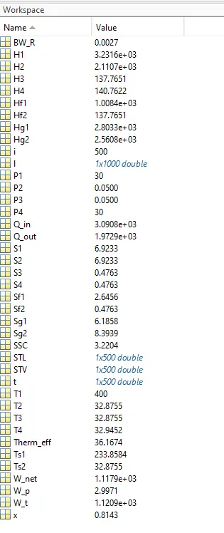
This the the screen shot of all the values in the workspace.
The output for each step in the command window is shown below.
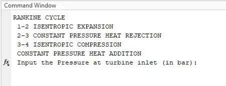
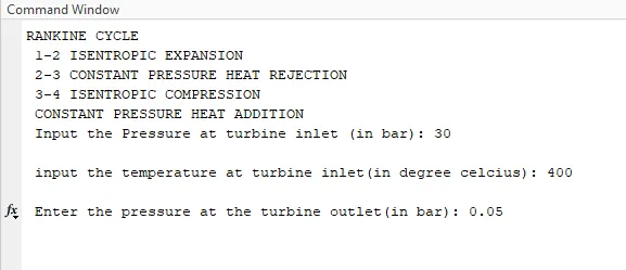
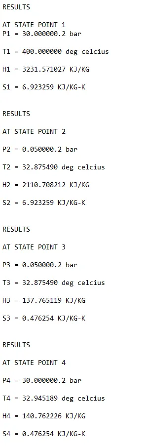
The final results as shown in the command window are displayed below
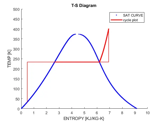
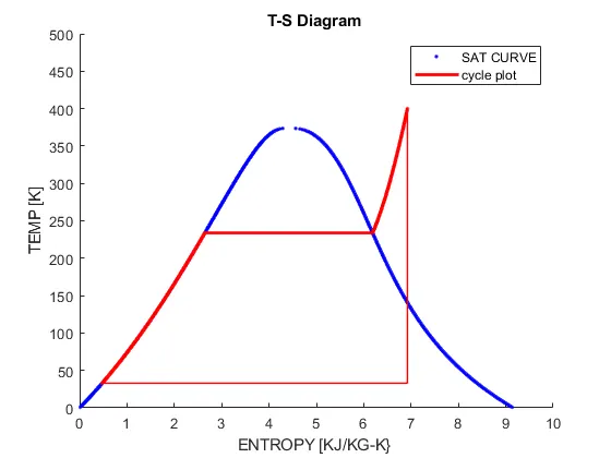
The below graph shows the T-S Diagram
The graph below shows the H-S graph.
ERRORS
This image below shows the error i got when i had not put in the variable P2. I had put P1 and the graph came out wrong.