Week 5.1 - Mid term project - Solving the steady and unsteady 2D heat conduction problem
AIM:-The aim of this project is to solve steady and unsteady 2D heat conduction
equation.
Matlab code:-
○ In the following program, we have solved equation(1) by using the iterative different
method which is mentioned above.
○ First, we have assumed that the number of grids in the x-direction is equal to the number of grids
in y-direction
○ And after that, we have initialized the array and assigning the boundary condition.
○ Then error and tolerance are set and the equation (1) solves one by one by
the different iterative methods in a loop.And each iterative method solve equation(1)
till convergence, the result is obtained.
○ After, the result is plotted using the contour command.
clear all
close all
clc
%Solving the steady 2D heat conduction equation
%Input parameter
nx=40; %no of grids in x-direction
ny=40; %no of grids in y_direction
rf=1.5; %relaxation factor
%Calculation
x=linspace(0,1,nx);
y=linspace(0,1,ny);
dx=x(2)-x(1); %Time step in x-direction
dy=y(2)-y(1); %Time step in y-direction
%Initializing array and assigning BC
T=ones(nx,ny);
T(:,1)=400;
T(1,:)=600;
T(:,end)=800;
T(end,:)=900;
Told=T;
%Constant
k=2*((dx^2+dy^2)/(dx^2*dy^2));
error=9e9; %error
tol=1e-4; %tolerance
iterative_solver=input
%Jacobi-method
tic
if iterative_solver==1
jacobi_iter=1;
while(error>tol)
for i=2:nx-1
for j=2:ny-1
H=(Told(i-1,j)+Told(i+1,j))/(dx^2);
V=(Told(i,j-1)+Told(i,j+1))/(dy^2);
T(i,j)=(H+V)/k;
end
end
error=max(max(abs(Told-T)));
Told=T;
jacobi_iter=jacobi_iter+1;
end
time1=toc;
figure(1)
colormap(jet)
contourf(x,y,T,':','showText','on')
xlabel('X axis')
ylabel('Y axis')
text1=sprintf('Number of iteration= %d',jacobi_iter);
text2=sprintf('Simulation time=%d s',time1);
title(['Steady state using jacobi_solver';text1;text2]);
colorbar
pause(0.3)
end
%Gauss seidal-method
tic
if iterative_solver==2
gs_iter=1;
while(error>tol)
for i=2:nx-1
for j=2:ny-1
H=(T(i-1,j)+Told(i+1,j))/dx^2;
V=(T(i,j-1)+Told(i,j+1))/dy^2;
T(i,j)=(H+V)/k;
end
end
error=max(max((abs(Told-T))));
Told=T;
gs_iter=gs_iter+1;
end
time2=toc;
figure(2)
colormap(jet)
contourf(x,y,T,'showText','on')
xlabel('X axis')
ylabel('Y axis')
text1=sprintf('Number of iteration= %d',gs_iter);
text2=sprintf('Simulation time=%d s',time2);
title(['Steady state using gs_solver';text1;text2]);
colorbar
pause(0.03)
end
%Successive overr relaxation-method
tic
if iterative_solver==3
sor_iter=1;
while(error>tol)
for i=2:nx-1
for j=2:ny-1
H=(T(i-1,j)+Told(i+1,j))/dx^2;
V=(T(i,j-1)+Told(i,j+1))/dy^2;
T(i,j)=Told(i,j)*(1-rf)+rf*((H+V)/k);
end
end
error=max(max(abs(Told-T)));
Told=T;
sor_iter=sor_iter+1;
end
time3=toc;
figure(3)
colormap(jet)
contourf(x,y,T,'showText','on')
xlabel('X axis')
ylabel('Y axis')
text1=sprintf('Number of iteration= %d',sor_iter);
text2=sprintf('Simulation time=%d s',time3);
title(['Steady state using sor_solver';text1;text2]);
colorbar
pause(0.03)
end
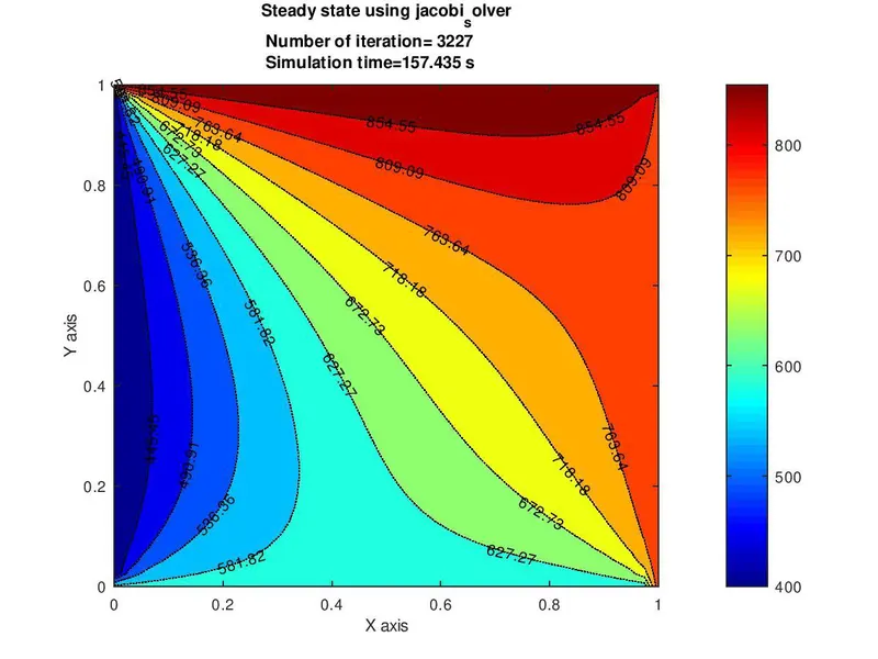
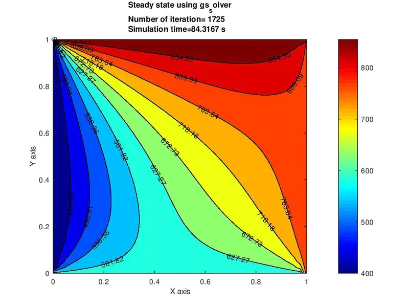
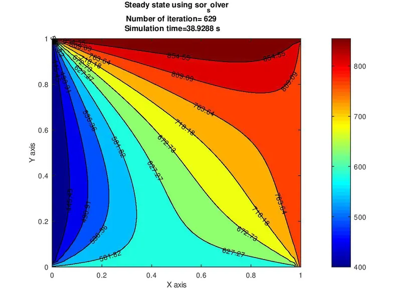
Result:-Following plots show the results for 2D heat conduction for steady-state using
different iterative methods.
Observation:-
○ While other two iterative solvers (Gauss seidel & Successive over-relaxation)
takes the updated values. Hence the new values are passed in a new iteration as the
solution proceeds. Thus in this type of iterative solver, we get convergence results
in less number iteration as well as in less computation time.
2. Solving 2D heat conduction equation for unsteady-state:-
Governing equation for the 2D heat conduction equation for the unsteady state is
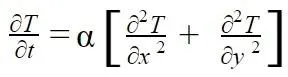
We will solve the above equation by using two schemes,
○ Explicit scheme
○ Implicit scheme
a.Explicit scheme:-
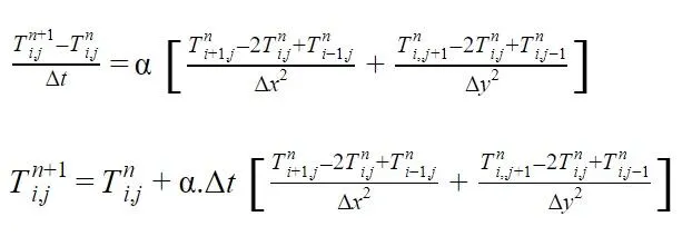
After applying for the first-order forward differencing scheme on L.H.S and central differencing
scheme on R.H.S on equation(2),we get
Let's say,
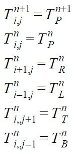
And, on simplification we get

Where k1 & k2 is,
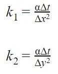
Equation (2) will be solved by using the point iterative method.The point iterative method
which will be used to solve the equation(2) are as follows:-
● Jacobi
● Gauss seidel
●Successive over-relaxation
Matlab code:-
○ In the following program, we have solved equation(3) by using different iterative
the method which is mentioned above.
○ First, we have assumed that number of grids in x-direction is equal to the number of grid
in y-direction
○ And after that, we have to initialize the array and assigning the boundary condition.
○ Then time loop is set in which equation (3) will be solved by using different
iterative method until the time loop gets to finish and convergence result is obtained.
○ After, the result is plotted using the contour command.
clear all
close all
clc
%Solving transient 2D heat conduction equation
%Input parameter
nx=40; %no of grids in x-direction
ny=40; %no of grids in y_direction
rf=1.5; %relaxation factor
dt=1e-4;
alpha=1.4;
nt=600;
%Calculation
x=linspace(0,1,nx);
y=linspace(0,1,ny);
dx=x(2)-x(1); %Time step in x-direction
dy=y(2)-y(1); %Time step in y-direction
%Initializing array and assigning BC
T=ones(nx,ny);
T(:,1)=400;
T(1,:)=600;
T(:,end)=800;
T(end,:)=900;
Told=T;
%Constant
k1=(alpha*dt)/(dx^2);
k2=(alpha*dt)/(dy^2);
iterative_solver=input
%Jacobi_iteration
if iterative_solver==1
tic
for k=1:nt % time loop
for i=2:nx-1
for j=2:ny-1
Term1=(1-2*k1-2*k2);
Term2=k1;
Term3=k2;
H=(Told(i-1,j)+Told(i+1,j));
V=(Told(i,j-1)+Told(i,j+1));
T(i,j)=(Told(i,j)*Term1)+(Term2*H)+(Term3*V);
end
end
Told=T;
end
time1=toc;
figure(1)
colormap(jet)
contourf(x,y,T,'showText','on')
colorbar
xlabel('x axis')
ylabel('Y axis')
text1=sprintf('Simulation time =%d s',time1)
title(['Transient state using jacobi';text1])
colorbar
pause(0.03)
end
if iterative_solver==2
%gs_iteration
for k=1:nt
for i=2:nx-1
for j=2:ny-1
Term1=(1-2*k1-2*k2);
Term2=k1;
Term3=k2;
H=(T(i-1,j)+Told(i+1,j));
V=(T(i,j-1)+Told(i,j+1));
T(i,j)=(Told(i,j)*Term1)+(Term2*H)+(Term3*V);
end
end
Told = T;
end
time2=toc;
figure(2)
colormap(jet)
contourf(x,y,T,'showText','on')
xlabel('X axis')
ylabel('Y axis')
text1=sprintf('Simulation time =%d s',time2)
title(['Transient state using gs_solver';text1])
colorbar
pause(0.3)
end
%sor_iteration
if iterative_solver==3
for k=1:nt
for i=2:nx-1
for j=2:ny-1
Term1=(1-2*k1-2*k2);
Term2=k1;
Term3=k2;
H=(T(i-1,j)+Told(i+1,j));
V=(T(i,j-1)+Told(i,j+1));
T(i,j)=Told(i,j)*(1-rf)+rf*((Told(i,j)*Term1)+(Term2*H)+(Term3*V));
end
end
Told = T;
end
time3=toc;
figure(3)
colormap(jet)
contourf(x,y,T,'showText','on')
xlabel('X axis')
ylabel('Y axis')
text1=sprintf('Simulation time =%d s',time3)
title(['Transient state using sor_solver';text1])
colorbar
pause(0.3)
end
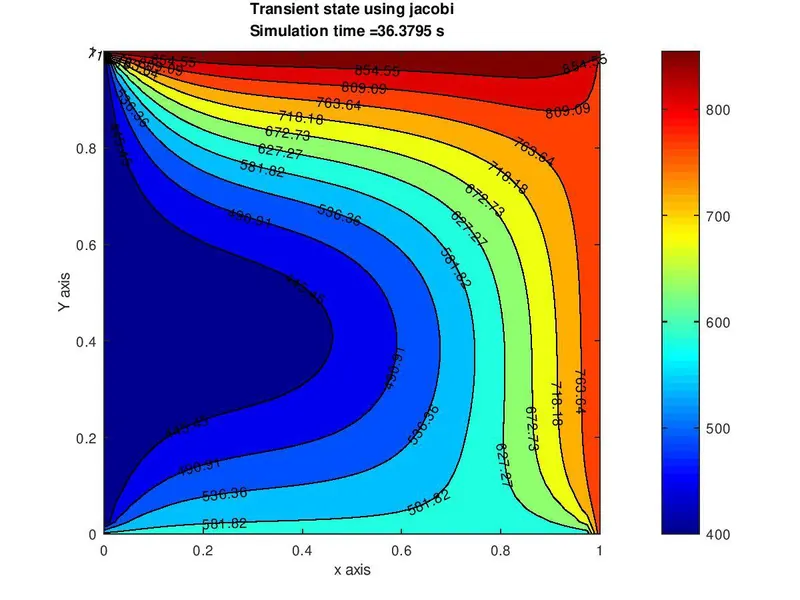
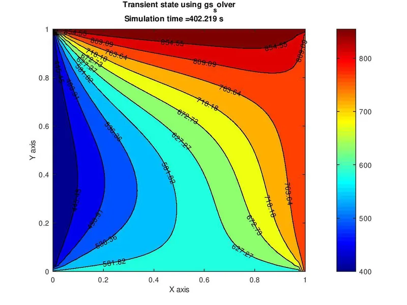
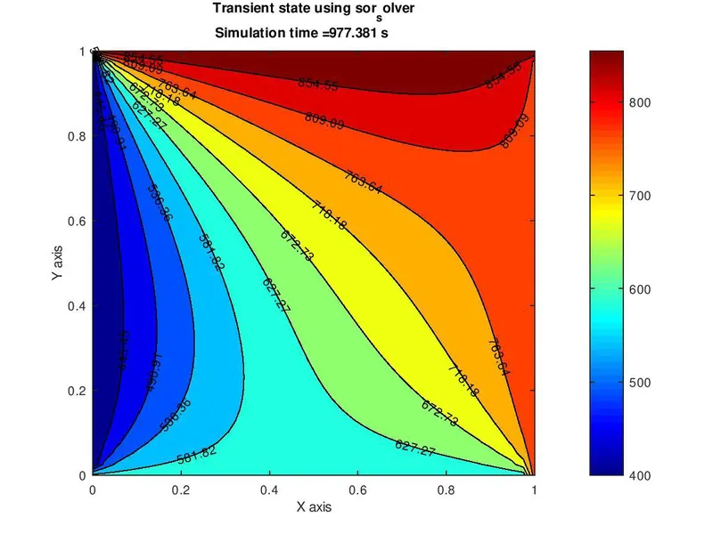
Result:-Following plots show the results for 2D heat conduction for Transient-state
explicit using different iterative methods.
Observation:-
○ By observing, above plots its quite clear that jacobi_iteration takes more number
of iteration and computation time as compared to the other two iterative solvers, this is
because the Jacobi method takes the old values.
○ While the other two iterative methods which are Gauss seidel & Successive over
relaxation iterative method shows most convergence result for the same value of
number of time steps as compared to the Jacobi method this is because Gauss
seidel & Successive over relaxation takes the updated values. Hence the new
values are passed in a new iteration as the solution proceeds. Thus in this type of
iterative solver, we get convergence result in less number of iteration as well as in
less computation time.
b. Implicit scheme:-
Governing equation for the 2D heat conduction equation for the unsteady state is,
We will solve the above equation by using two schemes,
○ Explicit scheme
○ Implicit scheme
a.Explicit scheme:-
After applying for the first-order forward differencing scheme on L.H.S and central differencing
scheme on R.H.S on equation(2),we get
Let's say,
And, on simplification we get
Where k1 & k2 is,

Equation (4) will be solved by using the point iterative method. The point iterative method
which will be used to solve the equation(4) are as follows:-
● Jacobi
● Gauss seidel
●Successive over-relaxation
Matlab code:-
○ In the following program, we have solved equation(4) by using different iterative
the method which is mentioned above.
○ First, we have assumed that the number of grids in the x-direction is equal to the number of grids
in the y-direction
○ Then error and tolerance are set in the time loop and then equation (4) is solved
one by one by different iterative methods in a loop. And each iterative method
solves equation(4) till convergence result is obtained.
○ After, the result is plotted using the contour command.
clear all
close all
clc
%Solving transient 2D heat conduction equation
%Input parameter
nx=40; %no of grids in x-direction
ny=40; %no of grids in y_direction
rf=1.5; %relaxation factor
dt=1e-3;
alpha=1.4;
nt=400;
%Calculation
x=linspace(0,1,nx);
y=linspace(0,1,ny);
dx=x(2)-x(1); %Time step in x-direction
dy=y(2)-y(1); %Time step in y-direction
%Initializing array and assigning BC
T=ones(nx,ny);
T(:,1)=400;
T(1,:)=600;
T(:,end)=800;
T(end,:)=900;
Told=T;
T_prev=T;
%Constant
k1=(alpha*dt)/(dx^2);
k2=(alpha*dt)/(dy^2);
error=9e9; %error
tol=1e-4; %tolerance
iterative_solver=input
tic
jacobi_iter=1
if iterative_solver==1
for k=1:nt
error=9e9;
while(error>tol)
for i=2:nx-1
for j=2:ny-1
Term1=(1+2*k1+2*k2)^-1;
Term2=k1*Term1;
Term3=k2*Term1;
H=(T(i-1,j)+Told(i+1,j));
V=(T(i,j-1)+Told(i,j+1));
T(i,j)=(T_prev(i,j)*Term1)+(Term2*H)+(Term3*V);
end
end
error=max(max(abs(Told-T)));
Told = T;
jacobi_iter=jacobi_iter+1
end
T_prev=T;
end
time1=toc;
figure(1)
colormap(jet)
contourf(x,y,T,'showText','on')
xlabel('X axis')
ylabel('Y axis')
text1=sprintf('Number of iteration =%d',jacobi_iter)
text2=sprintf('Simulation time =%d s',time1)
title(['Transient state using jacobi_solver';text1;text2])
colorbar
pause(0.3)
end
tic
gs_iter=1
if iterative_solver==2
for k=1:nt
error=9e9;
while(error>tol)
for i=2:nx-1
for j=2:ny-1
Term1=(1+2*k1+2*k2)^-1;
Term2=k1*Term1;
Term3=k2*Term1;
H=(T(i-1,j)+Told(i+1,j));
V=(T(i,j-1)+Told(i,j+1));
T(i,j)=(T_prev(i,j)*Term1)+(Term2*H)+(Term3*V);
end
end
error=max(max(abs(Told-T)));
Told = T;
gs_iter=gs_iter+1
end
T_prev=T;
end
time2=toc;
figure(2)
colormap(jet)
contourf(x,y,T,'showText','on')
xlabel('X axis')
ylabel('Y axis')
text1=sprintf('Number of iteration =%d',gs_iter)
text2=sprintf('Simulation time =%d s',time2)
title(['Transient state using gs_solver';text1;text2])
colorbar
pause(0.3)
end
tic
sor_iter=1
if iterative_solver==3
for k=1:nt
error=9e9;
while(error>tol)
for i=2:nx-1
for j=2:ny-1
Term1=(1+2*k1+2*k2)^-1;
Term2=k1*Term1;
Term3=k2*Term1;
H=(T(i-1,j)+Told(i+1,j));
V=(T(i,j-1)+Told(i,j+1));
T(i,j)=rf*((T_prev(i,j)*Term1)+(Term2*H)+(Term3*V))+(1-rf)*Told(i,j);
end
end
error=max(max(abs(Told-T)));
Told = T;
sor_iter=sor_iter+1
end
T_prev=T;
end
time3=toc;
figure(3)
colormap(jet)
contourf(x,y,T,'showText','on')
xlabel('X axis')
ylabel('Y axis')
text1=sprintf('Number of iteration =%d',sor_iter)
text2=sprintf('Simulation time =%d s',time3)
title(['Transient state using sor_solver';text1;text2])
colorbar
pause(0.3)
end
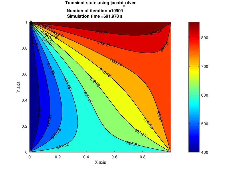
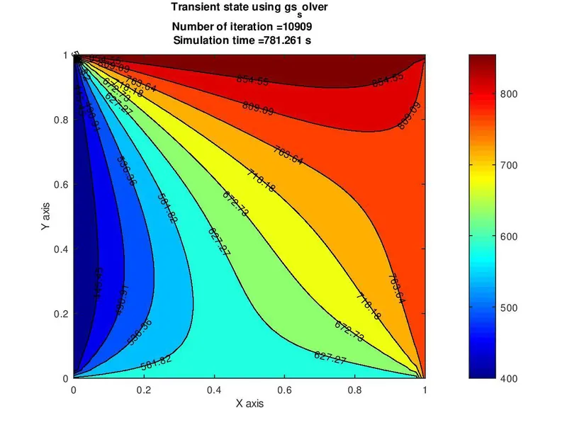
Result:-Following plots show the results for 2D heat conduction for Transient-state
an implicit scheme using different iterative methods.
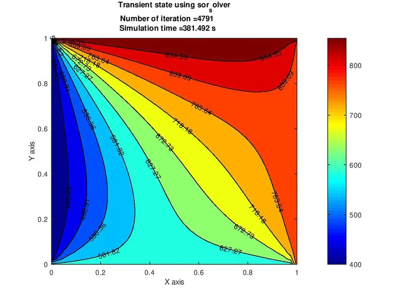
Observation:-
○ Tough we are getting the same result for different iterative methods so, the different
between them is the number of iteration and computation time taken by iterative
solver to get convergence results.