Week 6: Conjugate Heat Transfer Simulation

OBJECTIVE:

Baseline configuration

• Setup a flow simulation through a pipe
• Inlet Reynolds number should be 7,000
  • Re = (rho*V*D)/(Dynamic viscosity)
• Turbulence modelling - K-Epsilon
• Supercycling parameters - same as in the video

Additional 3D outputs

• Add Y+ to your post.in file

Grid dependence test

• Start with an initial base grid
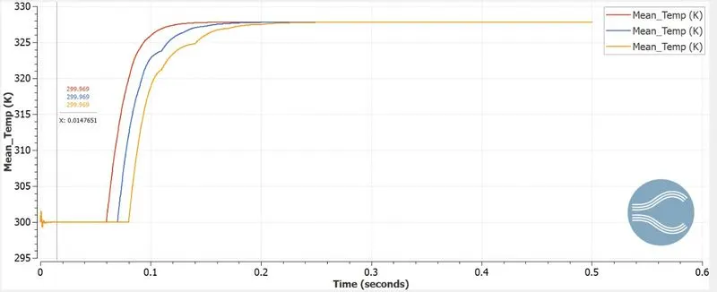
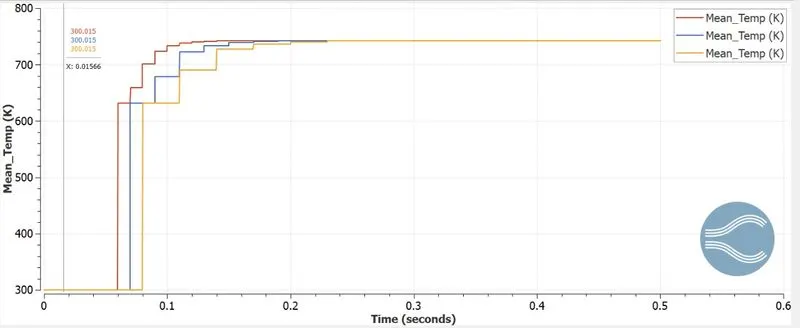
• Run grid dependence test on 3 grids and show that the outlet temperature converges to a particular value

Effect of supercycle stage interval

• Set supercyle stage interval to 0.01,0.02 and 0.03
• For these three values, how does the total simulation time compare against the baseline configuration.

THEORY:

The term conjugate heat transfer (CHT) is used to describe processes that involve variations of temperature within solids and fluids, due to thermal interaction between the solids and fluids. The exchange of thermal energy between the two physical bodies is called the study of Heat Transfer, the rate of transferred heat is directly proportional to the temperature difference between the bodies.

Conjugate heat transfer corresponds with the combination of heat transfer in solids and heat transfer in fluids. In solids, conduction often dominates whereas, in fluids, convection usually dominates. Efficiently combining heat transfer in fluids and solids is the key to designing effective coolers, heaters, or heat exchangers.

There different modes of heat transfer are namely:

1. Conduction: diffusion of heat due to temperature gradients. A measure of the amount of conduction for a given gradient is heat conductivity.

2. Convection: when the heat is carried away by moving fluid. The flow can either be caused by external influences, forced convection; or by buoyancy forces, natural convection. Convective heat transfer is tightly coupled to the fluid flow solution.

3. Radiation: transfer of energy by electromagnetic waves between surfaces with different temperatures, separated by a medium that is at least partially transparent to the (infrared) radiation. Radiation is especially important at high temperatures, e.g. during combustion processes, but can also have a measurable effect at room temperatures.

The major issue with conjugate heat transfer problems is that since modes of heat transfer is different, the timescales associated with the modes of heat transfer are different. Covective heat transfer happens relatively quickly, hence the fluid slover would be converging faster than the solver for the solid region. In order to eradicate this time scale disparity COVERGE STUDIO uses Super cycling.

Super cycling is a method used by CONVERGE Studio in the case of conjugate heat transfer problems with a solid and liquid region. The basic idea of super-cycling is that the solver for the fluid domain is paused until the solver for the solid domain converges. This pausing is done in intervals that can be set by the user and will be explained in the case setup.

To understand wall based phenomenon we need to look closely at the non dimensionless number Y+. This basically helps us understand where we exactly are in the boundary layer. This also helps us decide our first cell height. By keeping a value of Y+ between 0-5, we are in the viscous sub layer, between 5-10 we are in the transition region, and above 30 we are in the turbulent region of the boundary layer.

So by knowing Y+ we know how fine or coarse the grid should be, so that flow phenomenon close to the wall or away from it can be captured accurately. Also it helps us choose correct turbulence models.

SETUP:

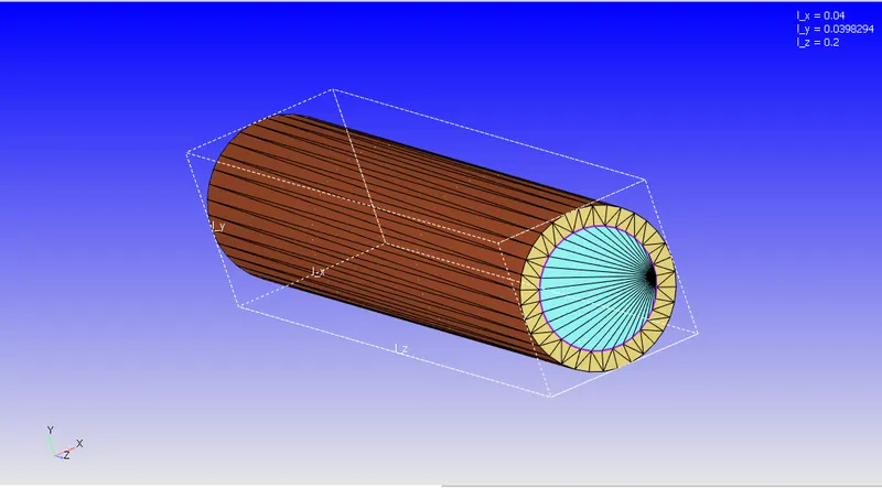
The geometry of the CHT model. Its important to we shall encounter non-manifold edges in CHT based simulations.

Application Type	Time-based
MATERIALS:
1. Gas simulation	Standard
2. Global Transport Parameters	Standard
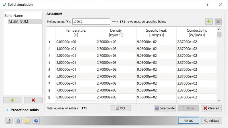
3. Solid simulation
4. Species	1. fluid: O2 and N2 2. Solid Aluminium
SOLUTION PARAMETERS
1. Run Parameters Steady-state monitor:	Transient >Full hydrodynamic>Compressible
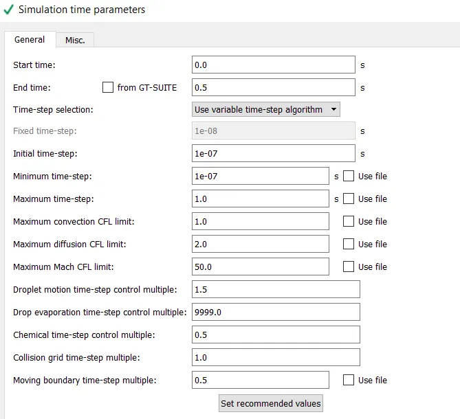
2. Simulation time parameters
3. Solver parameters	Navis-stokes solver scheme: PISO Navis-stokes solver type: density-based
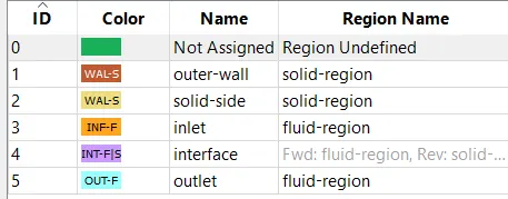
BOUNDARY CONDITIONS
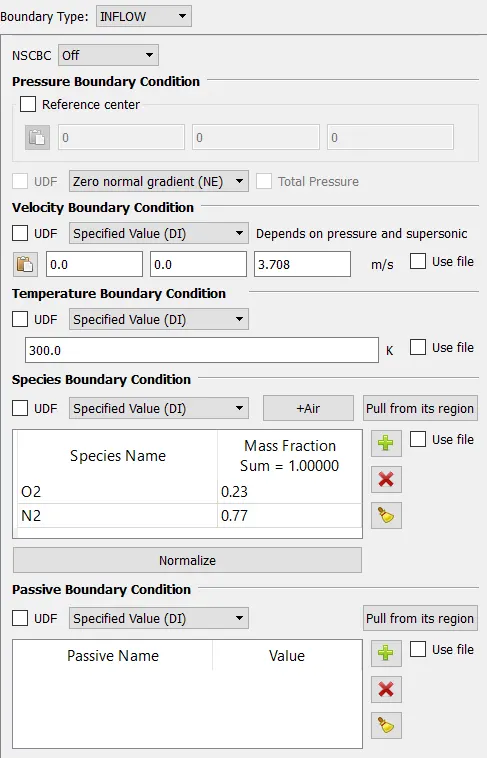
1. Inlet	Where: Re = 7000 velocity = 3.708 m/s
2. outlet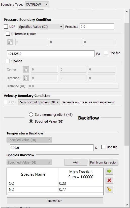
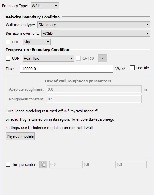
3. Outer wall
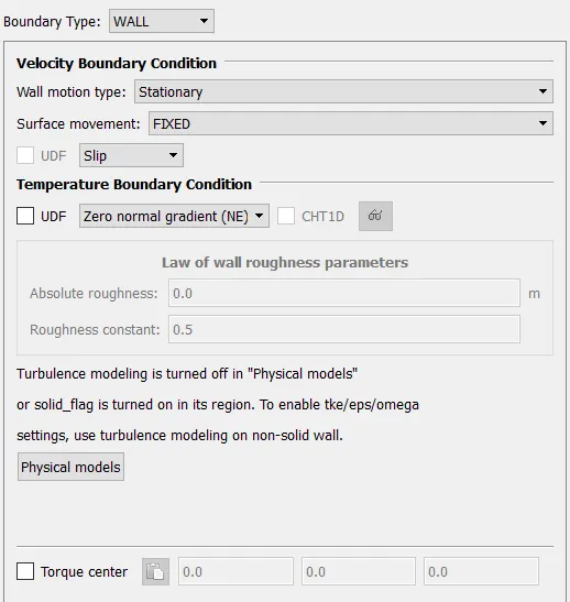
4. Side-wall
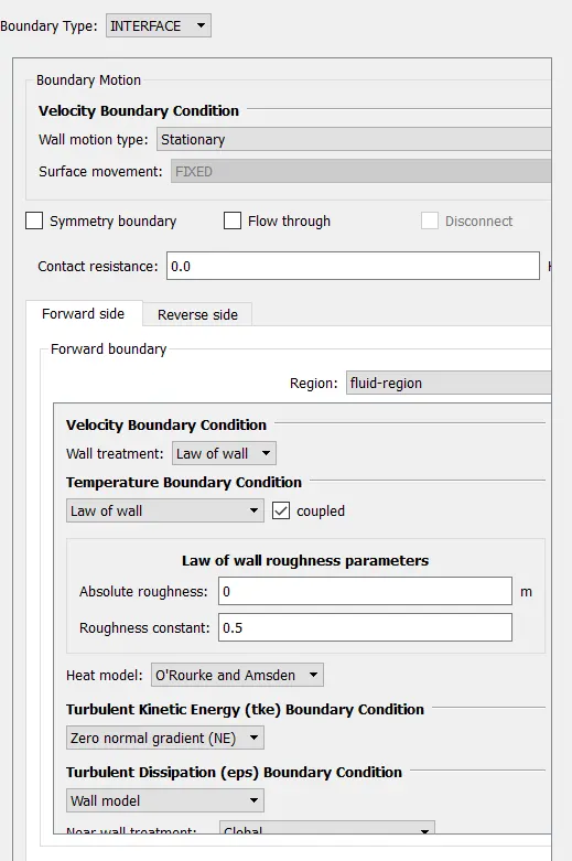
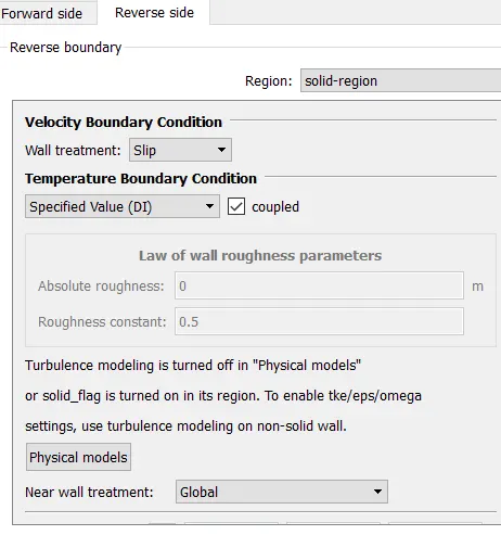
5. Interface
INITIAL CONDITIONS AND EVENTS
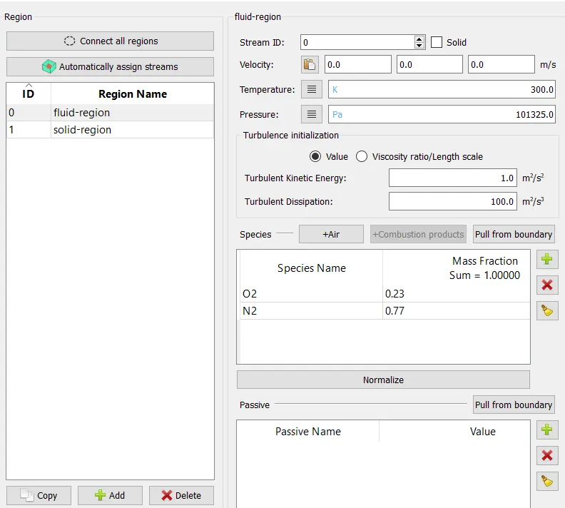
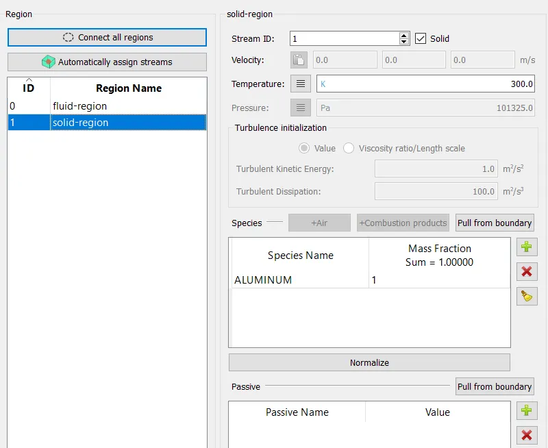
1. Regions and initialization
PHYSICAL MODELS
1 Turbulence modeling	RNG- k-epsilon
2. Super cycling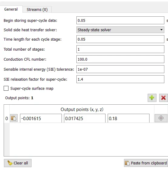
GRID CONTROL
1. Base mesh	CASE 1 dx = 0.004, dy = 0.004 and dz = 0.004 CASE 2 dx = 0.003, dy = 0.003 and dz = 0.003 CASE 3 dx = 0.002, dy = 0.002 and dz = 0.002
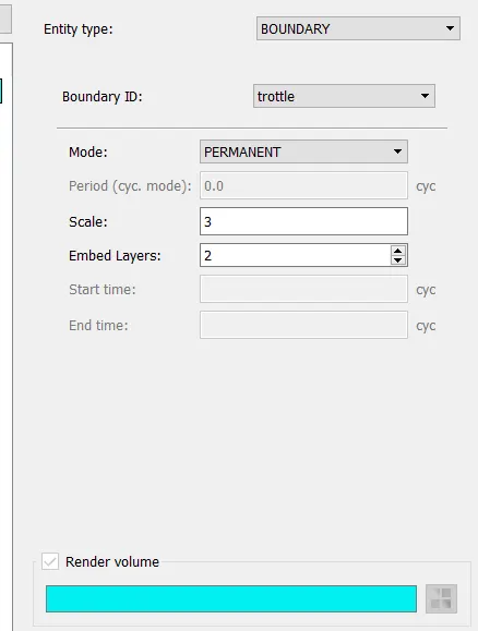
2. Fixed embedding
OUTPUT/POST-PROCESSING
1. Post variable selection	Add Y+
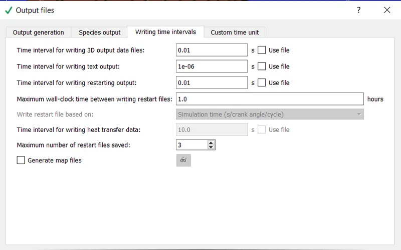
2. Output files:

RESULTS:

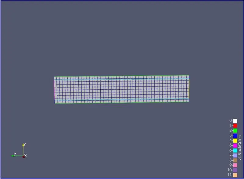
CASE-1 (0.04 mesh size)

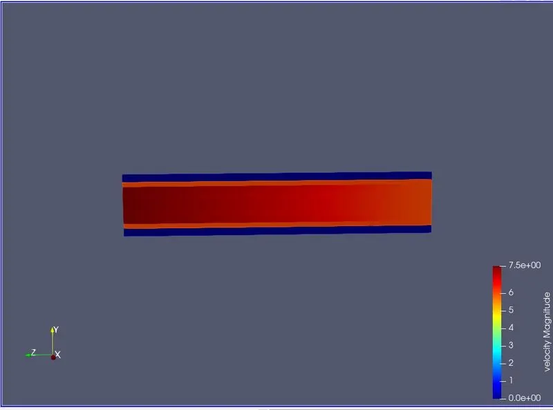
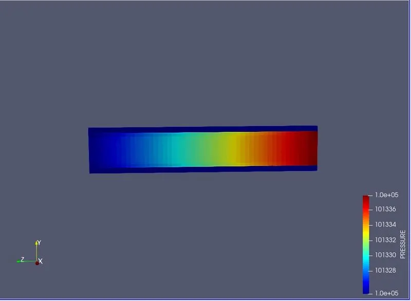
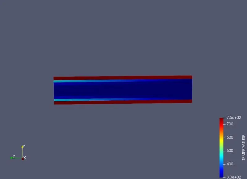
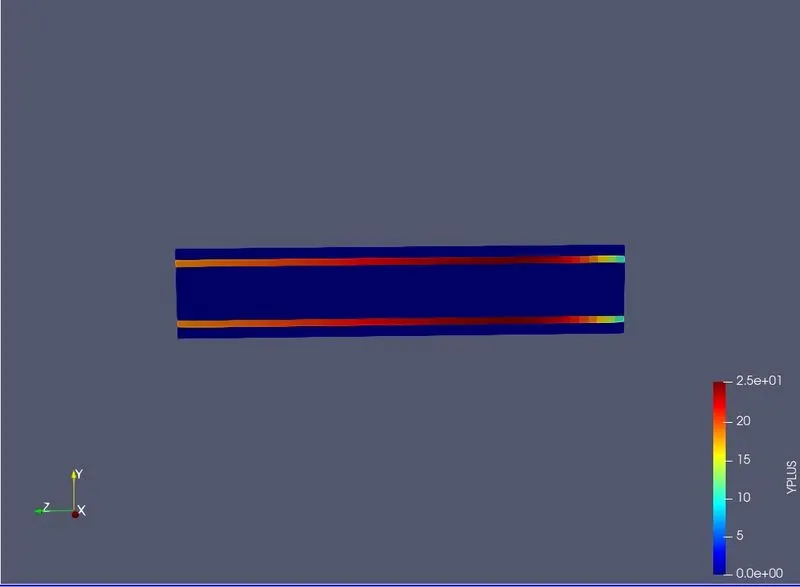
CASE-2 (0.03)

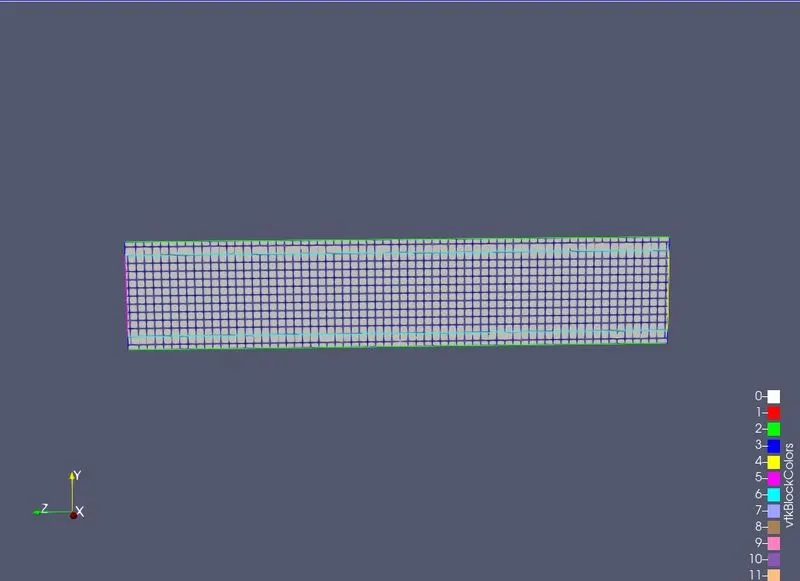
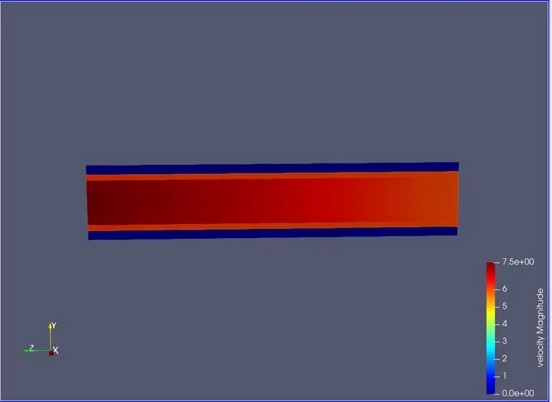
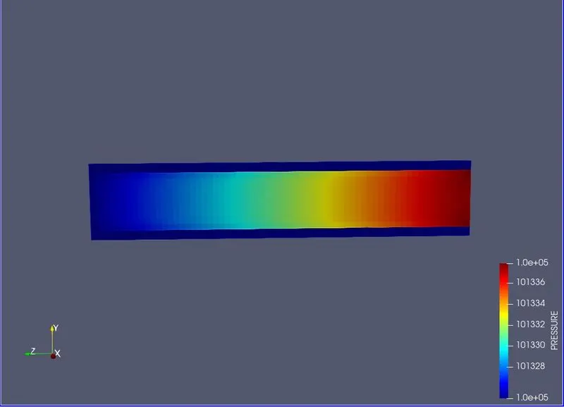
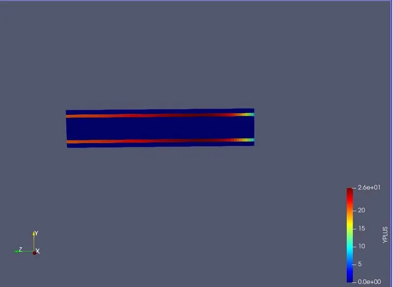
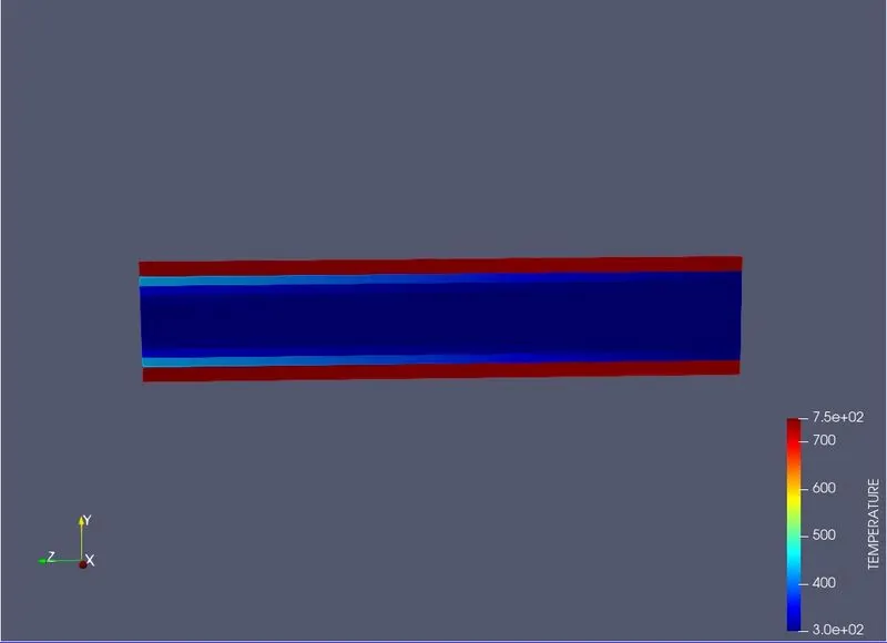
CASE-3 (0.02 mesh size)

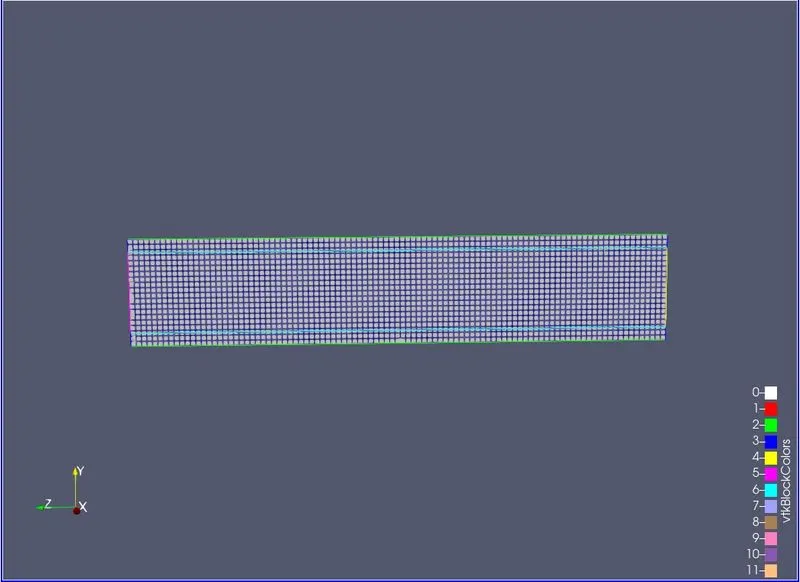
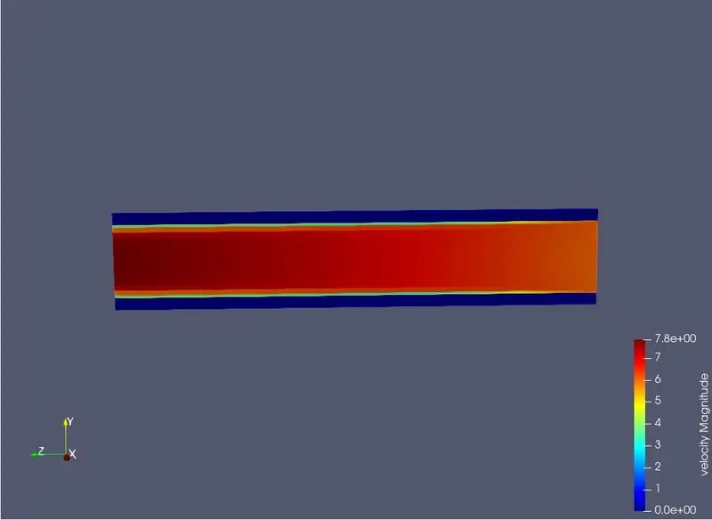
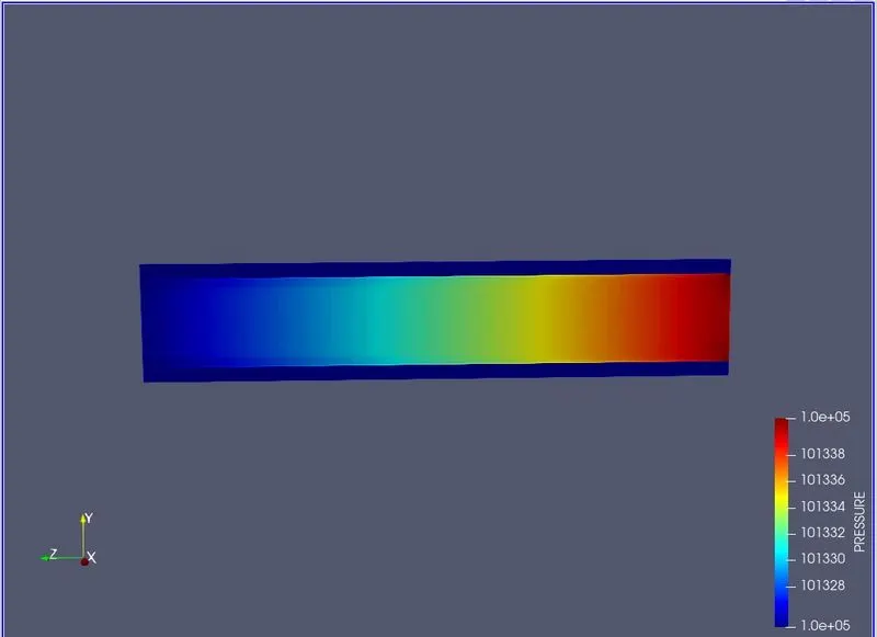
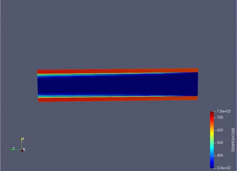
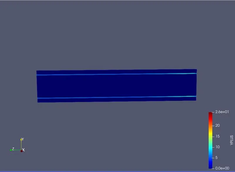
CASE-1 (Supercyling- 0.01)

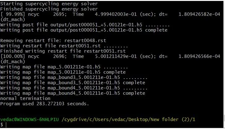
CASE-2 (Supercyling- 0.02)

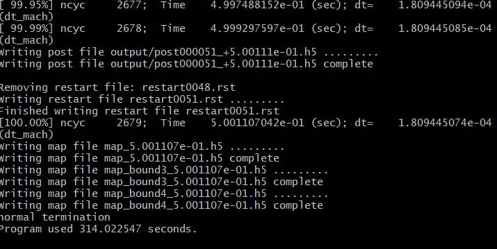
CASE-3 (Supercyling- 0.03)

FLUID REGION:

SOLID REGION:

CONCLUSIONS:

1. On looking into the grid dependence test we can see that finer the grid better the contours, more clear and distinct the phenomenon captured.

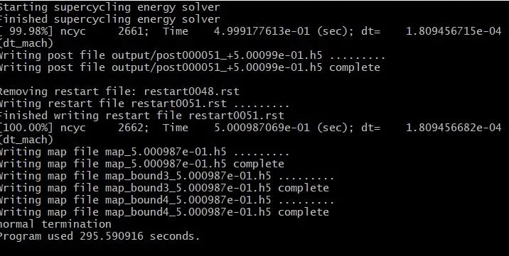
2. We see that keeping the supercycling values low the computational time reduces.