Week 7: Shock tube simulation project
OBJECTIVE:
1. Setup a transient shock tube simulation.
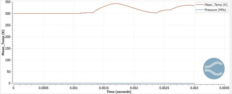
2. Plot the pressure and temperature history in the entire domain - Explain the result.
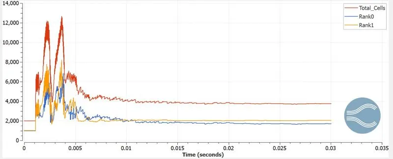
3. Plot the cell count as a function of time - Explain the result
THEORY:
The shock tube is an instrument used to replicate and direct blast waves at a sensor or a model in order to simulate actual explosions and their effects, usually on a smaller scale. They are a lab-scale device that is used to study shock movements, structures, etc.
They can also be used to study aerodynamic flow under a wide range of temperatures and pressures that are difficult to obtain in other types of testing facilities. Shock tubes are also used to investigate compressible flow phenomena and gas-phase combustion reactions.
A simple shock tube is a tube, rectangular or circular in cross-section, usually constructed of metal, in which gas at low pressure and gas at high pressure is separated using some form of a diaphragm. The diaphragm on bursting produces a wave propagating through the test section. The shock that eventually forms increases the temperature and pressure of the test gas and induces a flow in the direction of the shock wave.
The low-pressure gas is called the driven gas corresponding to the section is called the driven section, the high-pressure gas is called the driving gas, and the section is called the driving section.
The low-pressure gas is prefferd to be low molecular weight and a partial vacuum is maintained, so as to produce the strongest shocks.
There are various methods of bursting the diaphragm:
1. Using pyro-tech, for bursting
2. To use materials like plastic, which burst under specific pressures.
3. To use combustible mixtures, which create a detonation, hence causing a rupture.
Diagram showing the shock structure, in a simple shock tube.
A typical shock tube.
SETUP:
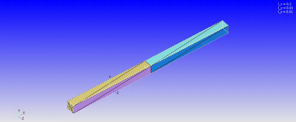
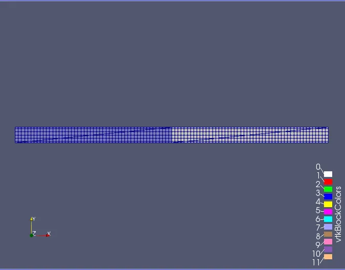
The mesh used for the simulation:
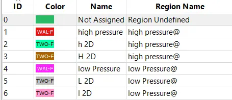
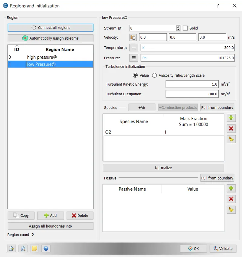
For the geometry prep, we need to form regions after appropriate boundary flagging. We need to define the high pressure and low-pressure regions very clearly, after running diagnosis, we conclude the geometry prep, by checking the normal orientation.
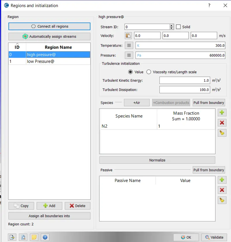
For our case, our driving gas is N2 (High pressure), and the driven gas is 02 (low pressure).
|
Application Type |
Time-based |
|
MATERIALS: |
|
|
1. Gas simulation |
Standard |
|
2. Global Transport Parameters |
Standard |
|
4. Species |
1. fluid: O2 and N2 |
|
SOLUTION PARAMETERS |
|
|
1. Run Parameters |
Transient >Full hydrodynamic>Compressible |
|
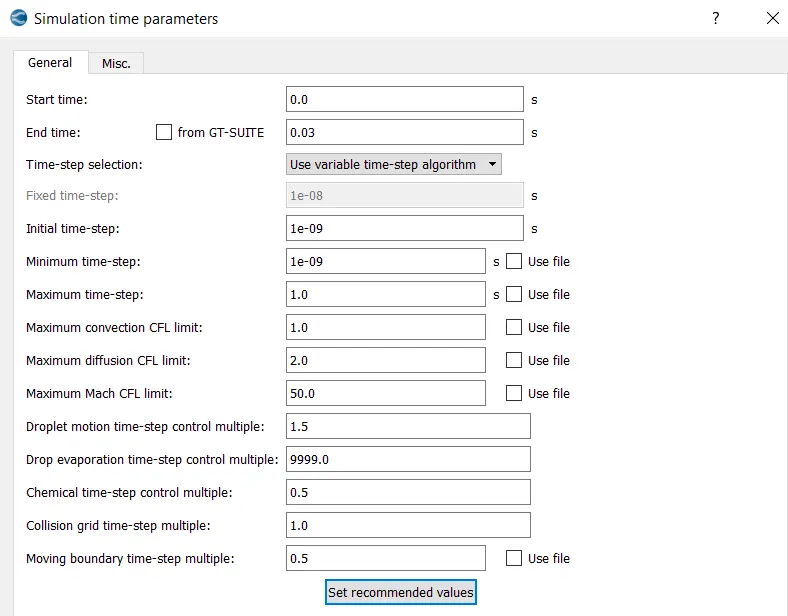
2. Simulation time parameters |
|
|
3. Solver parameters |
Navis-stokes solver scheme: PISO Navis-stokes solver type: density-based |
|
BOUNDARY CONDITIONS |
 |
|
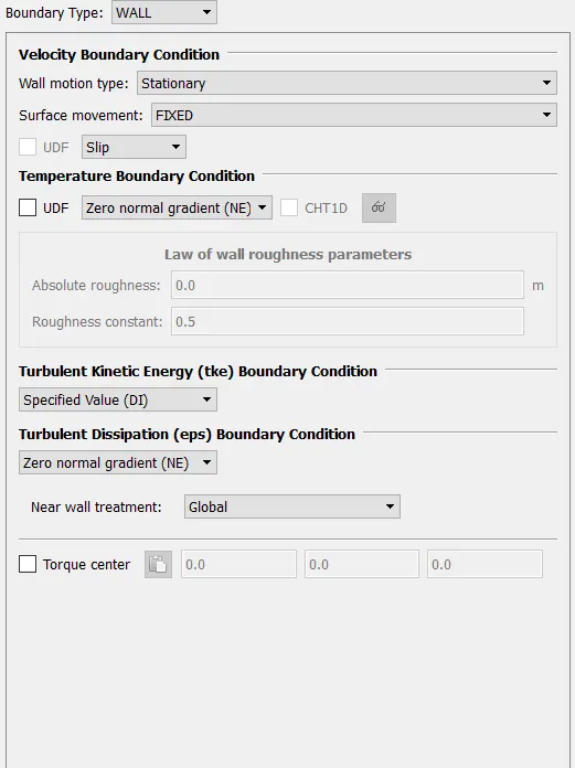
1. High-pressure wall |
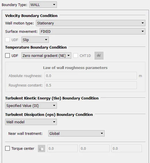 |
| 2. High-pressure 2D front and Back | 2D wall |
|
3. Low-pressure wall |
 |
|
4. Low-pressure 2D front and back wall |
2D wall |
|
INITIAL CONDITIONS AND EVENTS |
|
|
1. Regions and initialization |
|
|
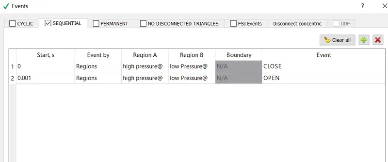
2. EVENTS |
 |
|
PHYSICAL MODELS |
|
|
1 Turbulence modeling |
RNG- k-epsilon |
|
GRID CONTROL |
|
|
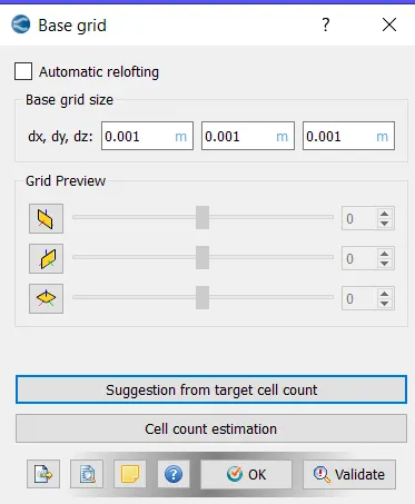
1. Base mesh |
|
|
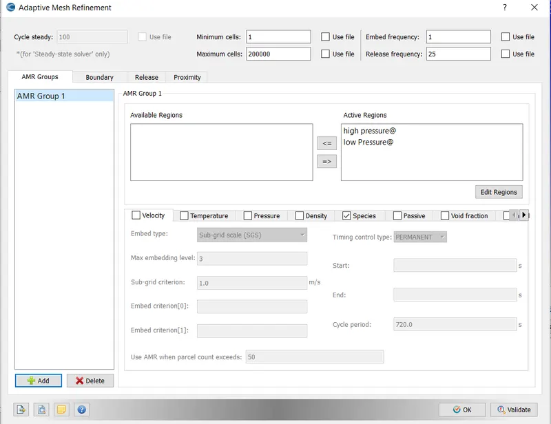
2. Adaptive meshing |
|
|
OUTPUT/POST-PROCESSING |
|
|
1. Post variable selection |
Standard |
|
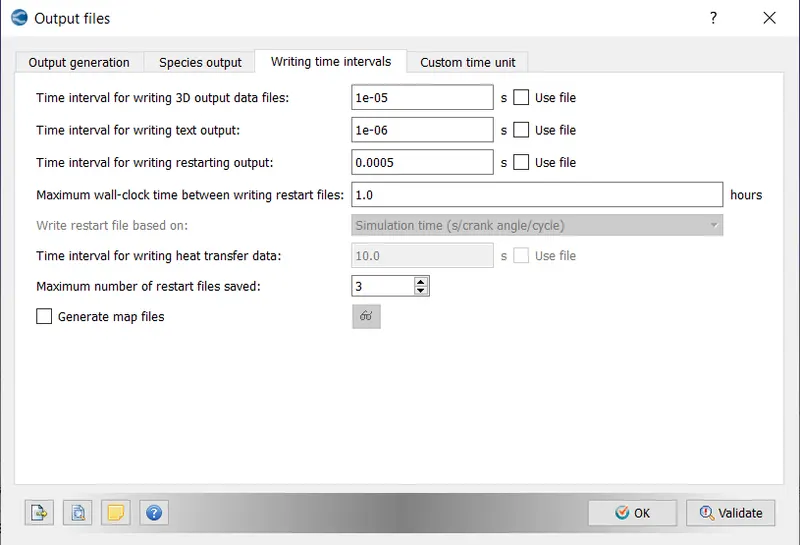
2. Output files: |
|
RESULTS:
The contours for the velocity, temperature, and pressure is given below:
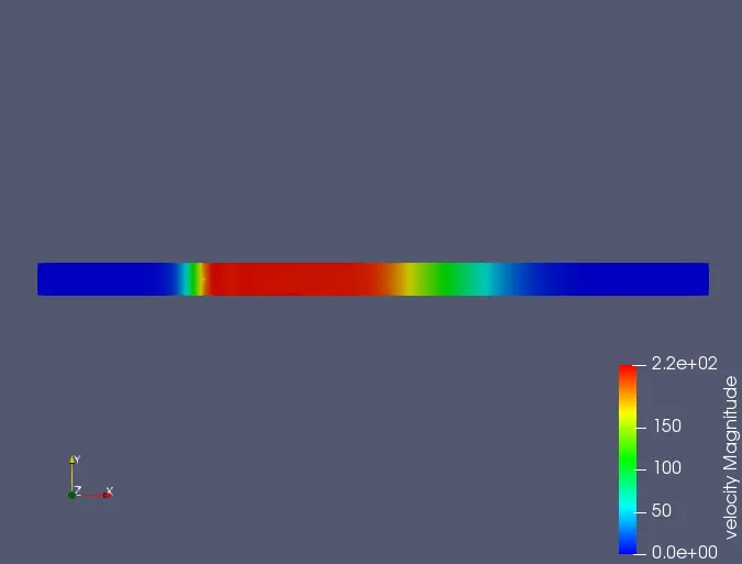
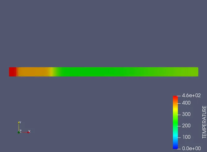
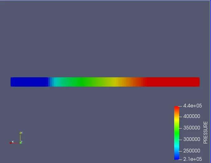
PRESSURE PLOTS
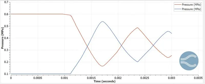
TEMPERATURE
CELL COUNT
Velocity, temperature & pressure video links are attached below
CONCLUSIONS:
1. High-pressure N2 compresses the low pressure 02 then after compression, a recirculation takes place.
2. The shock tube helps us understand the compressibility of gases.
3. The AMR settings help us capture the shock waves and recirculation regions that we see behind the wake
4. The temprature contours are a bit different we see the temprature distribution more gradual than pressure and velocity before it reaches equilibrium.