Week 5 - Rayleigh Taylor Instability

OBJECTIVE:

1. To find some practical CFD models that have been based on the mathematical analysis of Rayleigh Taylor waves.
2. Perform the Rayleigh Taylor instability simulation for 2 different mesh sizes with the base mesh being 0.5 mm. [Using air-water mixture for simulation]
3. Run one more simulation with water and user-defined material(density = 400 kg/m³, viscosity = 0.001 kg/m-s) for refined mesh.
4. Define the Atwood Number. Find out the Atwood number for both the cases and explain how the variation in Atwood number in the above two cases affects the behavior of the instability.

THEORY:

Rayleigh-Taylor instability is an important phenomenon in fluid mechanics that has applications from very basic and mundane things like oil on water to nuclear explosions and structures of pulsars and supernovas. It is basically about the instability of an interface between two fluids having different densities, where the lighter fluid is pushing the heavier one.

The basic mechanism of this instability is that the denser fluid on top, due to acceleration due to gravity, creates a perturbation, where the heavier fluid is displaced downward, which results in the lighter fluid of equal volume being, pushed upward. This upward push causes an increase in potential energy, and consequently on observing this cycle we see that the perturbation keeps growing.

The initial perturbations follow a linear progression, after which the amplitude of the perturbation increases non-linearly, in the non-linear phase, non-linear models are required as amplitudes are large. In brevity, the density disparity determines the structure of the R-T instability.

Apart from R-T instability, there are few more known in fluid mechanics.

Ritchmyer-Meshkov Instability:

This instability arises, when there is a shock at the interface of liquids. This includes the impulsive acceleration of fluids of different densities. This has a linear trend of perturbation followed by a non-linear trend with bubbles appearing in the case of a light fluid penetrating a heavy fluid and with spikes appearing in the case of a heavy fluid penetrating a light fluid.

Plateau-Rayleigh Instability:

This instability describes why a stream of water, breaks down into droplets, the same fluid volume but just lesser surface area. The primary driving force for this instability is surface tension which tends to minimize their surface area. Concepts of wave numbers further determine the number of droplets etc. Used in inkjet technologies where ink is converted into tiny droplets.

Kelvin-Helmhotz instability:

This instability generally occurs when two streams of fluid are set in opposite directions. Owing to some perturbations and Bernoulli's theorem, there is a pressure increase in a region and a subsequent decrease in another. This results in the region of fluid risen to be caught up by the stream forming interesting patterns. We see them in clouds, wind over waves, or on the Jupiter surface.

PRACTICAL CFD MODELS

SPH (Smooth particle hydrodynamics):

This method is used to simulate the mechanics of continuous media, such as solid mechanics and fluid mechanics. It is a mesh-free model which has its own set of advantages. The main advantage is that it's well suited for complex boundary phenomena, free-surface flows, and boundary displacements. The model implementation is easier, computational cost per unit particle is lesser. The main disadvantage of this method is setting up boundary conditions like inlet and outlet.

SINGLE FLUID MODEL:

In this model, two distinct phases are considered a mixture and are considered to flow as a mixture, with 5 equations describing the system, with mass, momentum, energy, and the other two describing the phases involved.

TWO FLUID MODEL:

In a two-phase model apart from describing the two district phases as a single mixture, the governing equations are distinct. The interaction of the interface (heat transfer) is not taken into consideration. The velocity slip between two phases is taken into consideration.

TURBULENCE:

These models have employed to simulate the mixing behavior of two phases. They can be solved for simple cases, but for most practical applications they predict the evolution of turbulence. These models are simplified so that they can be solved to predict evolution.

SETUP

1. Open space claim, draw two 20x20mm squares which are on top of each other, it's necessary to convert them into a surface.

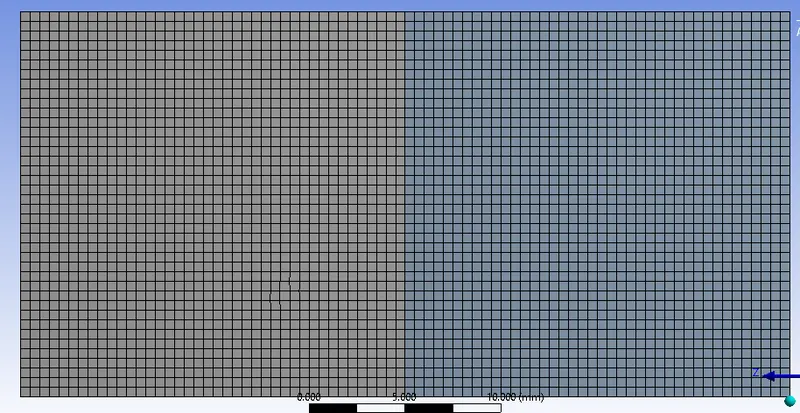
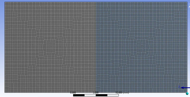
2. Open meshing and we need to simulate the following cases, only changing element size, kept smoothing at high.

These are the mesh statistics.

CASES	NODES	ELEMENTS
0.5mm (BASE)	3321	3200
0.3mm	9180	8978
0.1mm	80601	80000
0.2mm( USER-DEFINED)	20301	20000

3. The fluent set-up has to be done as follows:

a.Transient state has to be switched on, with gravity enabled, an acceleration of -9.8m/s^2. in the y-direction.

b. Multiphase option turned on, with volume extract and implicate method. Two Eulerian phases selected.

c. The primary and secondary phases have to be described.

d. In material properties, the appropriate setting of phases has to be done with corresponding parameters.

e. Hybrid initialized with proper patching done. Ensure the correctness of the set-up by phase plots of water.

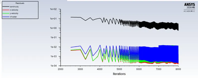
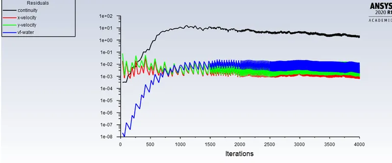
f. Time steps size=0.001s, No of time steps=800, Time-step/iteration approx=10.

RESULTS AND DISCUSSIONS:

CASE-1 (BASELINE 0.5mm)

ANIMATION:

https://drive.google.com/file/d/1lLKnLKNP35okBi-G-lMfFQKZT_49wu0x/view?usp=sharing.

This the 0.5mm animation.

CASE-II

0.3mm

ANIMATION:

https://drive.google.com/file/d/1H1KJRSSiqoo6-vFRnsWFnuhMNIhcHIEe/view?usp=sharing

This is the 0.3mm grid size animation.

CASE-III

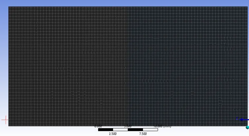
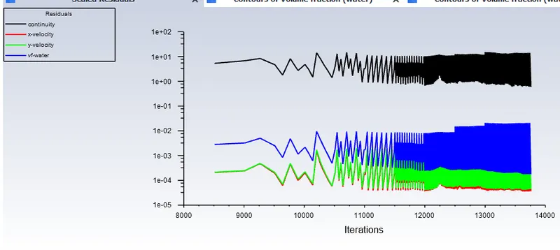
0.1mm ( Fine-Mesh)

ANIMATIONS:

https://drive.google.com/file/d/1REZWea00mFlwc0obiUUdcNfbR6ph1eS6/view?usp=sharing

0.1mm is the mesh size.

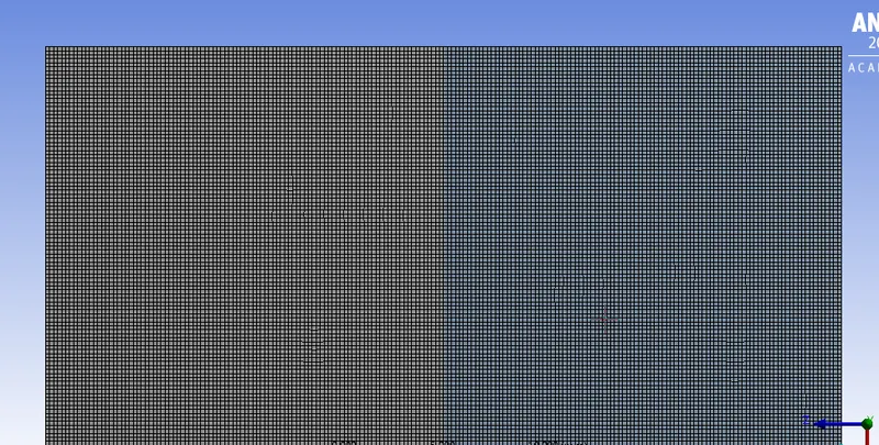
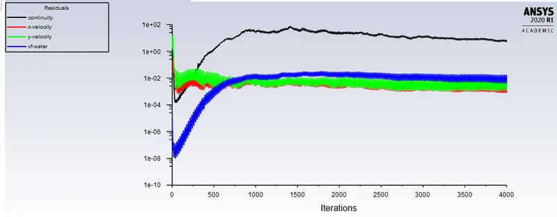
CASE-IV ( User-defined material)

ANIMATION:

https://drive.google.com/file/d/1_47LzeRAgTXBGcn-wbcw-YYuH0E_C4D0/view?usp=sharing

This the user-defined case, with mesh size used as 0.2mm.

CALCULATION:

Atwood number is a dimensionless number that is used for studying hydrodynamic instabilities in density stratified flows. Mathematically defined as:

where

= density of heavier fluid

= density of the lighter fluid

The penetration distance of the bubble is a function of Agt^2, where A is the Atwood number, this is directly related to the growth of the instability. Also, the structure of the subsequent instability is given by this number, for Atwood number close to zero the instability looks like symmetric fingers, and closer to 1 the lighter fluid below the heavier one take shape of a plume or mushroom cloud.

FOR CASE I, II, III:

A=998.2-1.225/(998.2+1.225)

A=0.9975

FOR USER DEFINED CASE:

A=998.2-400/(998.2+400)

A=0.4278

So when water is poured over the lighter fluid, the air pushes the heavier media and forms plume-like bubbles. This also an important parameter in Ritchmyer-Meshkov Instability.

We can see the individual animations of each case in comparison with the Atwood number, we see that the plume-like contours are visible since the Atwood number is close to 1. In the user-defined material, the Atwood number is about 0.5, the inherent plume characteristics still persist, the mixing pattern looks a bit different from the previous cases.