Week 4.1: Project Steady state simulation of flow over a throttle body

OBJECTIVE:

To simulate a steady state flow around a throttle body, to produce the pressure velocity contours, also to produce the plots for the flow variables.

THEORY:

Throttling in engineerring system design is an important design feature when control over power or engine output is an important part of the problem statement. In a broad sense it can be defined as process of regulating the output of the power source by regulating the input.

In many engineering applications this regulation is done by regulating the fuel input to the power generating source, the mass flow rate of the fuel can be controlled so that a corresponding output is generated.

In liquid propusion systems, the flow of propellents to the combustion chamber is regulated through a network of valves and plumbing systems, in automobiles we see valves which are attached to accleration mechanism, which regulates the fuel flow to the engine system.

A throttle body is essentially an air valve that sits between the intake manifold and air intake pipe, it regulates the amount of air going into the engine which is crucial for the fuel/air ratio.

The throttle body for our simulation is a bent hollow cylindrical pipe, with a throttle plate. A throttle shaft passes through the body, which is attached to the controlling or acclerating mechanism. By the movement of the throttle plate we can regualte the fluid flow.

STEADY STATE ANALYSIS:

In our simulation we shall be performing steady state analysis, where the flow variables do not change with respect to time. Basically the phenmomen of accumulation is ruled out, we do not compute how long it takes for the system to reach steady state.

SETUP:

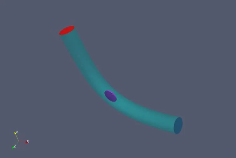
This is the 3D model of the throttle body, we can see the throttle plate or disc, coloured purple.

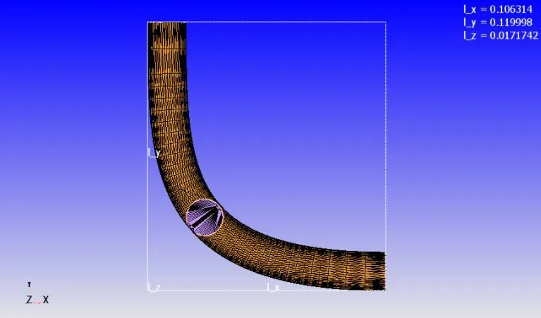
Geometry imported as STL file in coverge studio.

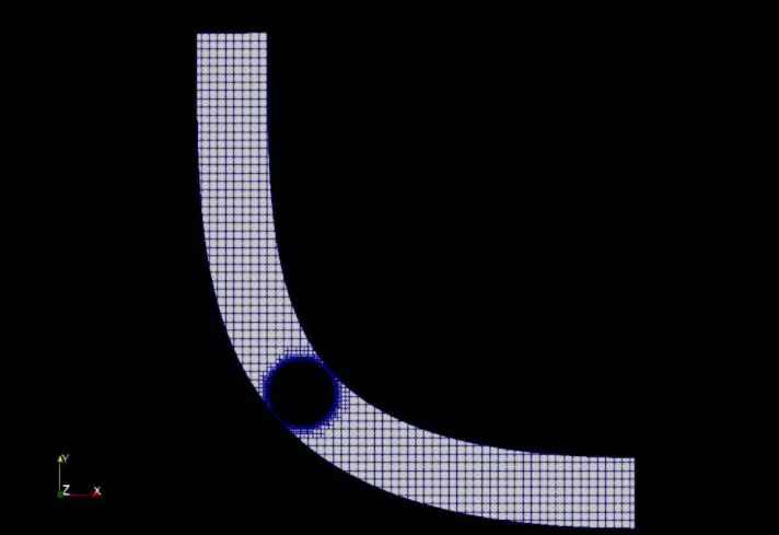
This the mesh, we can clearly see the baseline mesh, and a fixed embedding aroung the throttle body.

Application Type	Time-based
MATERIALS:
1. Gas simulation	Standard
2. Global Transport Parameters	Standard
3. Reaction Mechanism	Standard
SOLUTION PARAMETERS
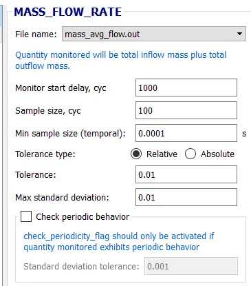
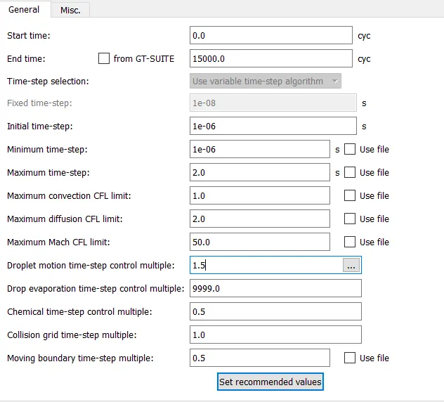
1. Run Parameters Steady-state monitor:	Steady-state solver>Full hydrodynamic>Compressible Mass flow rate
2. Simulation time parameters
3. Solver parameters	Navis-stokes solver scheme: PISO Navis-stokes solver type: pressure-based Max convection CFL limit: 0.5
BOUNDARY CONDITIONS
1. Inlet
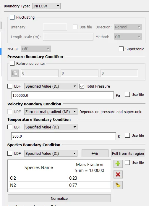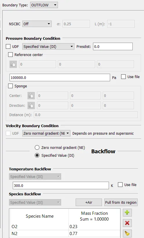
2. Outlet
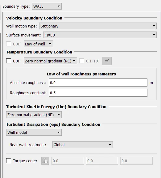
3. Elbow-wall
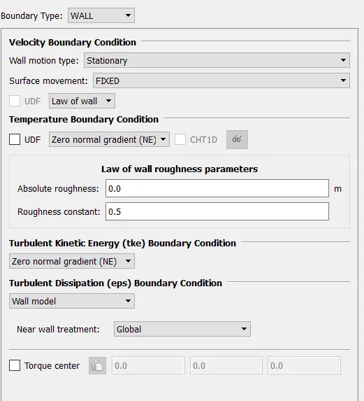
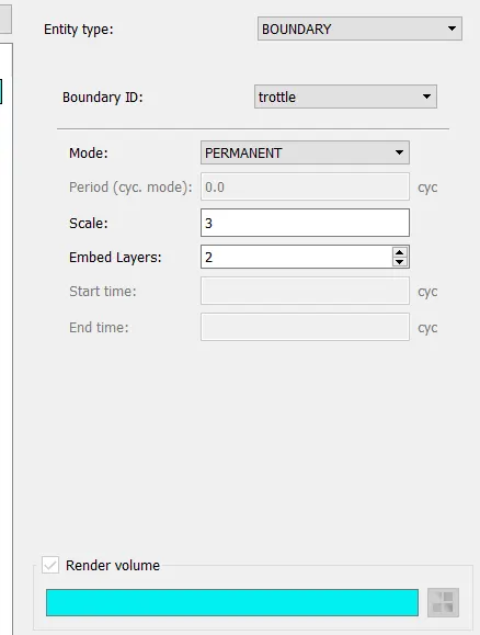
4. Throttle
INITIAL CONDITIONS AND EVENTS
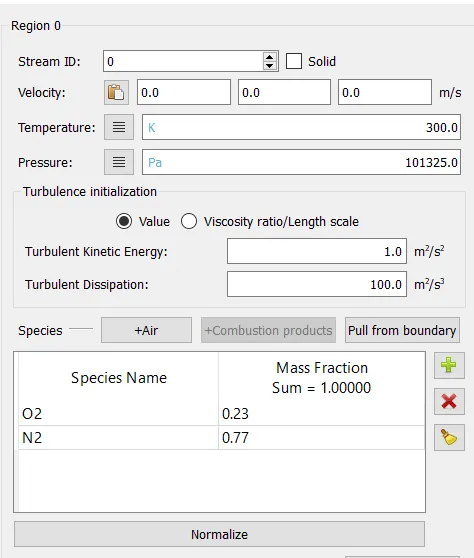
1. Regions and initialization
PHYSICAL MODELS	RNG- k-epsilon
GRID CONTROL
1. Base mesh	dx = 2e-3m, dy = 2e-3m and dz = 2e-3m
2. Fixed embedding
OUTPUT/POST-PROCESSING
1. Post variable selection	Standard
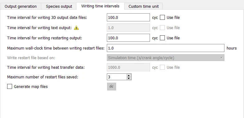
2. Output files:

RESULTS:

The contours for pressure and velocity is shown below

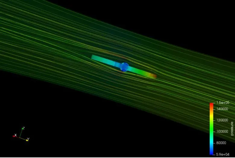
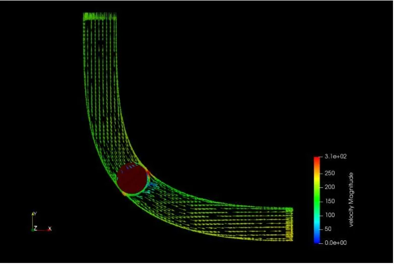
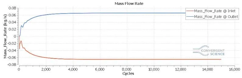
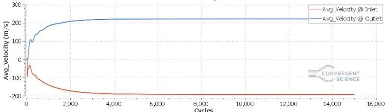
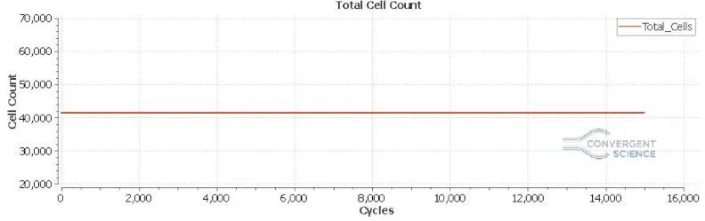
The plots for mass flow rate, velocity and cell count is shown

CONCLUSIONS:

1. The fixed embedding near the wall, enables us to capture the flow around the throttle body with great resolution, as the cell count is increased.

2. At the circumfrence of the plate adjacent to the wall we see that the velocity is highest, owing to low flow area and low pressure.

3. The point of incidence of the flow and the throttle plate, shows highest pressure as it is the stagnation point and the velocity is least in that region.

4. Also at the curved protrusion at top we can see high velocity.