Week 10: Modeling and Simulation of flow around an Ahmed Body
OBJECTIVE:
- Create the CAD model using your any CAD package
- Setup a Coarse CFD simulation
- Setup the virtual wind tunnel as shown in the video
- Apply the right boundary conditions and solver settings
- Use a coarse mesh to demonstrate that your setup runs successfully.
- You need to show an animation of the velocity distribution on a cutplane. This cutplane should cut the ahmed body model in two symmetric pieces.
- You need to show an animation of the pressure distribution on a cutplane. This cutplane should cut the ahmed body model in two symmetric pieces.
- Post process the coarse mesh results and extract the x component of velocity along a line(Here, I am assuming that the normal of the intake boundary is along the +x direction)
- The line should be perpendicular to the ground plane.
- Enable wall-averaged outputs to measure the drag and lift forces
- Calculate the steady state drag force value and explain your calculation procedure.
- Calculate the drag co-efficient using paraview and explain your calculation process in detail
You should explain your simulation approach by providing appropriate technical information.
THEORY:
As the burning of fossil fuels becomes a more pressing issue, manufacturers are introducing more fuel efficient cars to the market. One main contributor to fuel burn is the car’s aerodynamic drag. Complexly shaped, cars are very challenging to model and it’s difficult to quantify the aerodynamic drag computationally. The Ahmed body is a benchmark model widely used in the automotive industry for validating simulation tools. The Ahmed body shape is simple enough to model, while maintaining car-like geometry features.
The drag quantifies the resistance of an object in a fluid environment. It is not an absolute constant for a body’s shape because it varies with the speed and direction of flow, object shape and size, and the density and viscosity of the fluid. The lower the drag coefficient of an object, the less aerodynamic or hydrodynamic drag occurs. In terms of a car, the lower the drag coefficient, the more efficient the car is. As well as affecting the top speed of a vehicle, the drag coefficient also affects the handling. Cars with a low drag coefficient are sought after, but decreasing the drag drastically can reduce the downforce and lead to loss in road traction and a higher chance of car accidents. So a design tradeoff becomes necessary keeping the problem statement in mind.
The total drag coefficient of the Ahmed body is the key measurement for this simulation. It is made up of measurements for the pressure coefficients in the front, slant, and base of the body as well as the body’s skin friction. The recirculation and wake region is captured at the end.
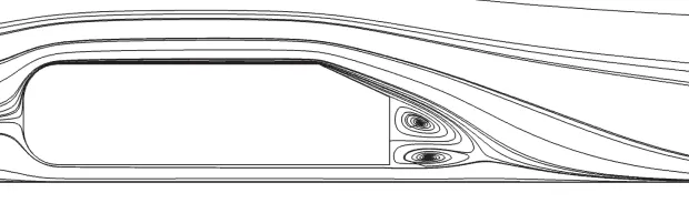
Due to the sudden change in slope, the flow attached to surface observes the no-slip and has lesser velocity, the flow which is seperated has higher momentum, this forms a high pressure region and the flow forms a circulatory region at the aft.
SETUP:
This is the standard geomerty made on a CAD package.
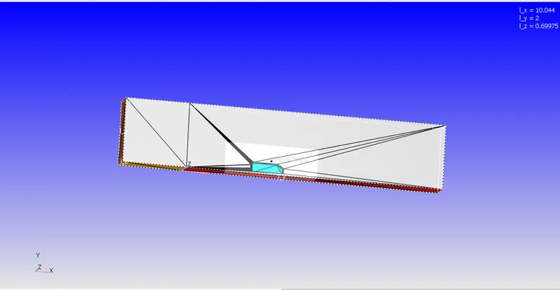
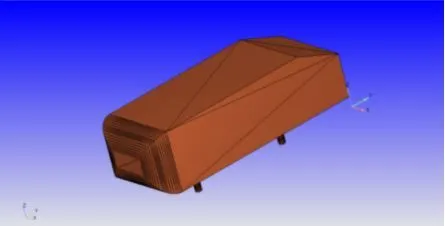
The geometry of Ahemed body is shown in closeup as a STL file.
SETUP:
|
Application Type |
Time-based |
|
MATERIALS: |
|
|
1. Gas simulation |
Standard |
|
2. Global Transport Parameters |
Standard |
|
4. Species |
O2 and N2 |
|
SOLUTION PARAMETERS |
|
|
1. Run Parameters |
Transient >Full hydrodynamic>Compressible |
|
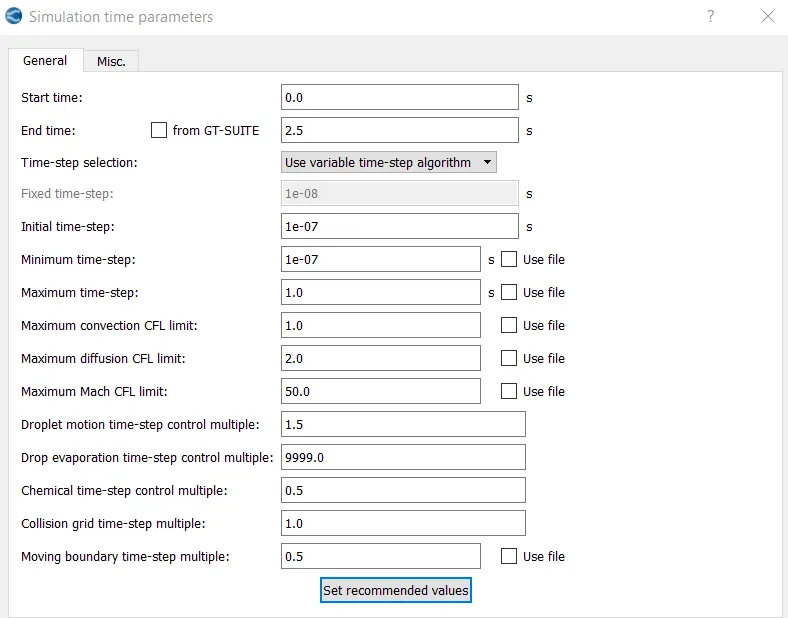
2. Simulation time parameters |
|
|
3. Solver parameters |
Navis-stokes solver scheme: PISO Navis-stokes solver type: density-based |
|
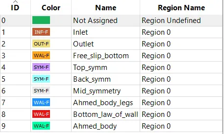
BOUNDARY CONDITIONS |
 |
|
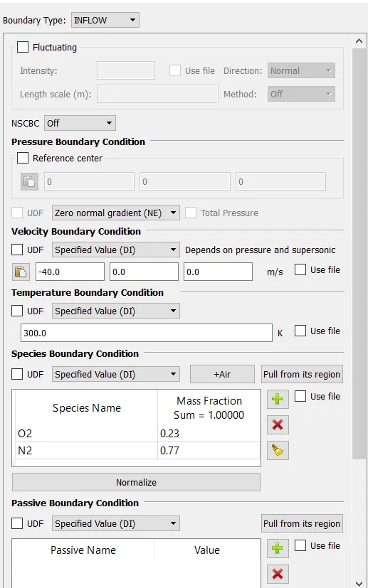
1. Inlet |
|
| 2. Outlet | 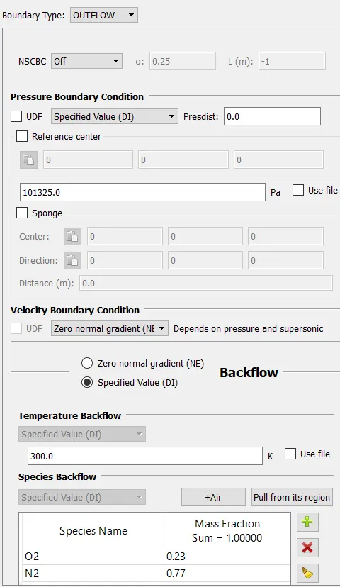 |
|
3. free_slip_bottom |
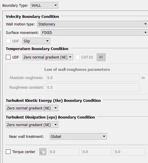 |
|
4. Top_symmetry |
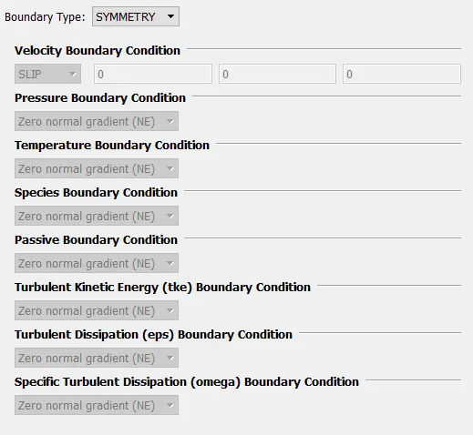 |
|
5. Back_symmetry |
|
|
6.Mid_symmetry |
|
|
7. Ahmed body legs |
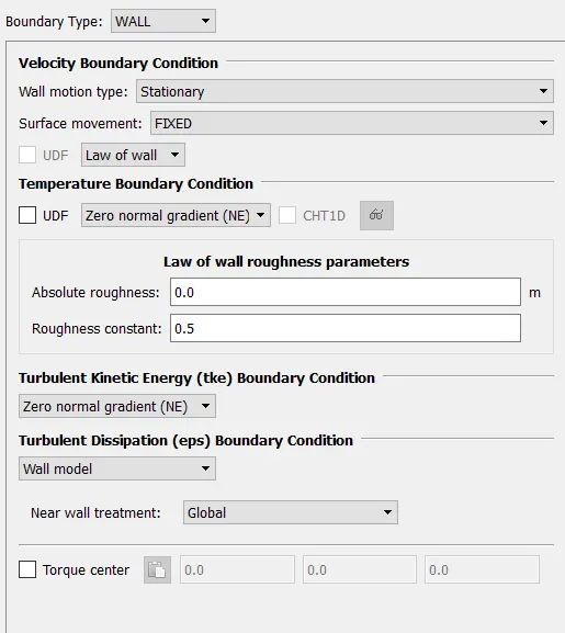 |
|
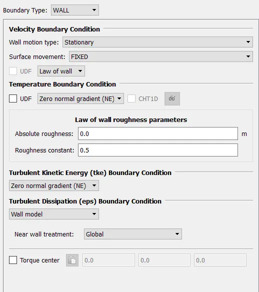
8. Bottom law of wall |
 |
|
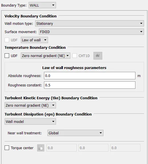
9. Ahemd body |
 |
|
INITIAL CONDITIONS AND EVENTS |
|
|
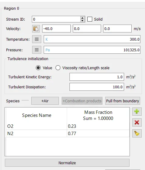
1. Regions and initialization |
|
|
PHYSICAL MODELS |
|
|
1 Turbulence modeling |
RNG-k-epsilon |
|
GRID CONTROL |
|
|
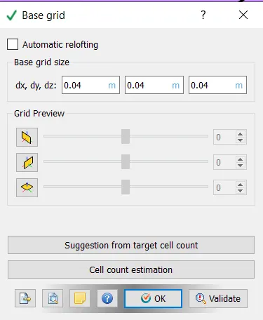
1. Base mesh |
|
|
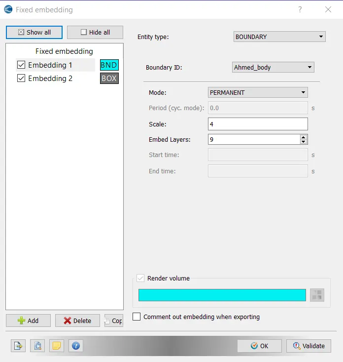
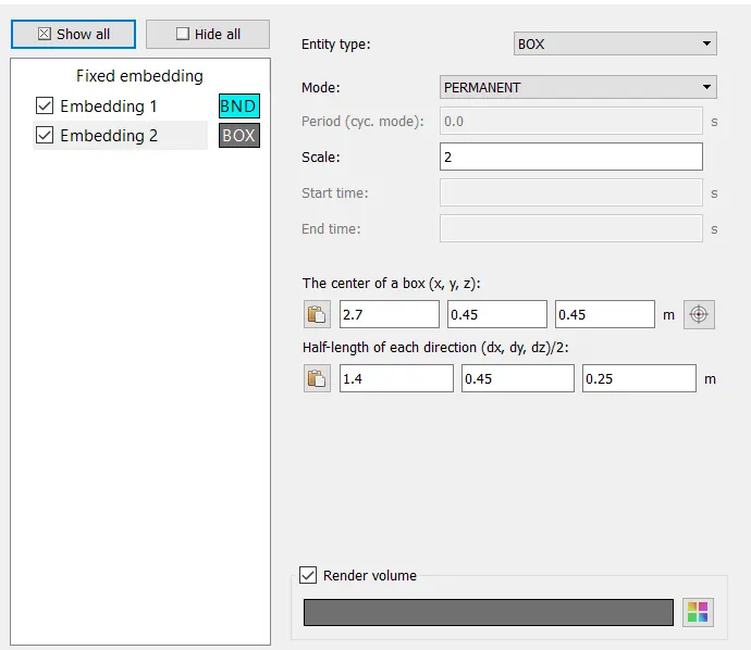
2. Fixed meshing |
|
|
OUTPUT/POST-PROCESSING |
|
|
1. Post variable selection |
Standard |
|
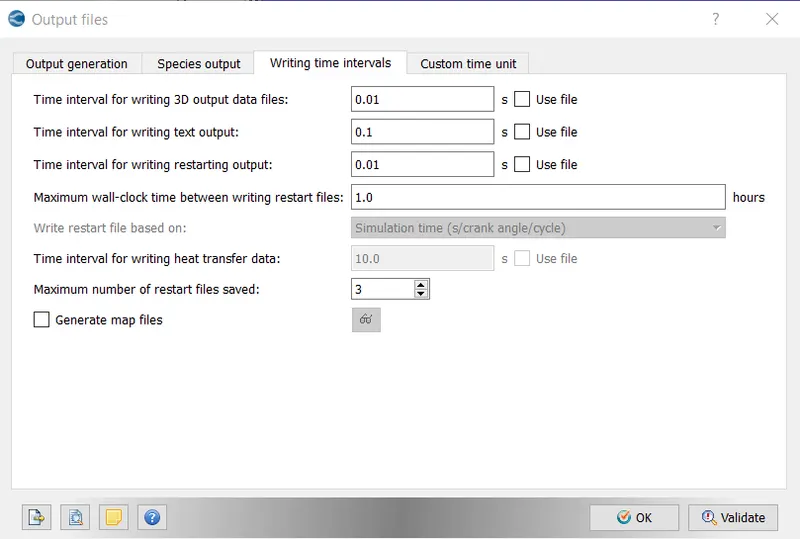
2. Output files: |
|
RESULTS:
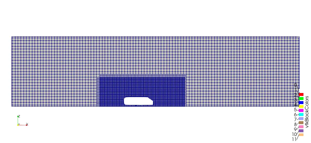
The mesh used for the simulation.
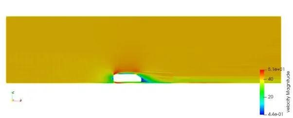
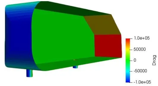
The blue region at the aft of the ahmed body, showing regions of flow seperation, with the recirculatory wake
region at the aft of the body, this recircualtory region is responsible for increased pressure drag.
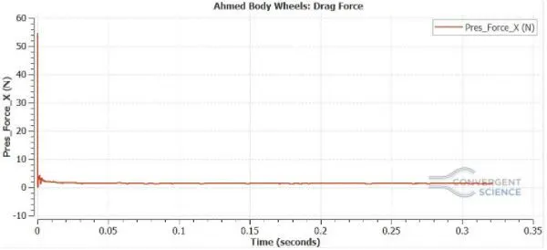
The coefficent of drag can be calculated as
D=5.25 N
Cd= 5.25*2/1.225*40^2*(0.22*0.38)
Cd=0.064
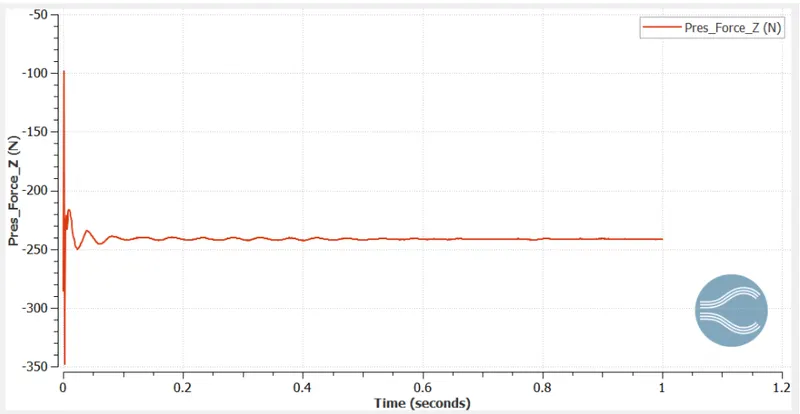
The coefficent of lift can be calculated as
L=-240 N
Cd= -240*2/1.225*40^2*(0.22*0.38)
Cd=-2.92
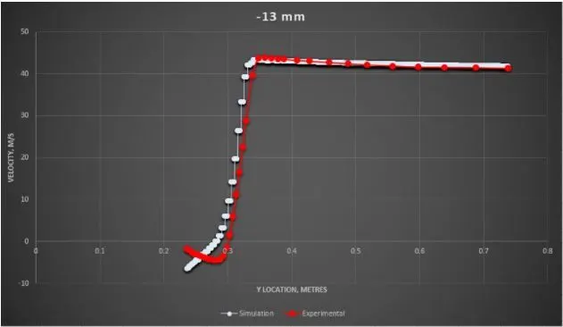
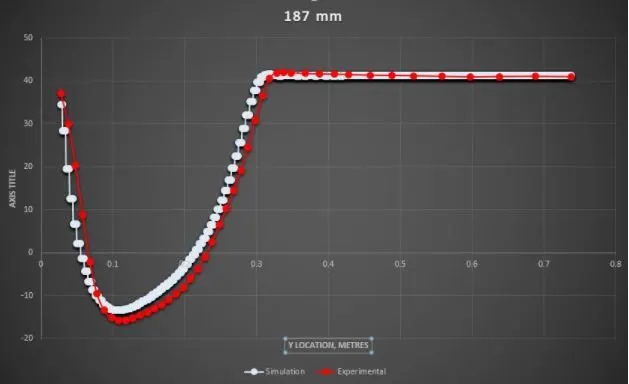
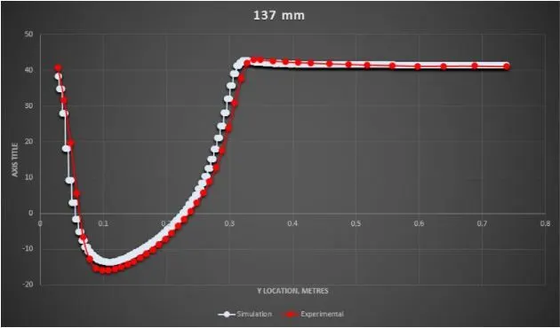
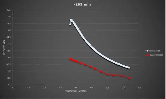
The probe line plots showing variance of velocity with respective spatial axis, an experimental and computational plots are compared. The probes are located in different loactions.
CONCLUSIONS:
1. The experimental and computational values show decent agreement.
2. The error on the postive side is greater as most of the wake region and drag is produced.
3. To capture the wake region we need finer grid size.
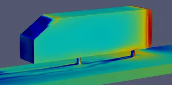
4. The flow coming from the cylindrical stands, there are vortices that are observed from a top view
5. The lift generated is negative, this is the required down force to maintain traction.