Week 8 - Simulating Cyclone separator with Discrete Phase Modelling

OBJECTIVE OF SIMULATION:

1. To write a few words about any four empirical models used to calculate the cyclone separator efficiency.
2. To perform an analysis on a given cyclone separator model by varying the particle diameter from 1 μm to and calculate the separation efficiency in each case.
3. To perform an analysis on a given cyclone separator model by varying the particle velocity from 1 m/sec to 5 m/sec and calculate the separation efficiency and pressure drop in each case.

THEORY:

A cyclone separator is an economical device for removing particulate solids from a fluid system. The induced centrifugal force is tangentially imparted on the wall of the cyclone cylinder. This force, with the density difference between the fluid and solid, increases the relative settling speed. In simple words, it utilizes principles of inertia, for the separation of particles, heavier particles having more inertia, hence through centrifuge action, they settle down with the lighter ones rising with an upward draft type of flow.

A spinning gas stream separates particles from the carrier gas. Their simple design, low capital cost, and nearly maintenance-free operation make them ideal for use as pre-cleaners for more expensive final control devices like electrostatic precipitators. Cyclones are particularly well suited for high temperature and pressure conditions because of their rugged design and flexible component materials. Cyclone collection efficiencies can reach 99% for particles bigger than 5 µm, hence they can be used for rugged conditions and high dust loading. The one used in our study is the tangential rectangular inlet.

The flow field inside a cyclone separator is swirl-dominated, with specific characteristics in radial, axial & tangential directions, we look at it a bit more closely.

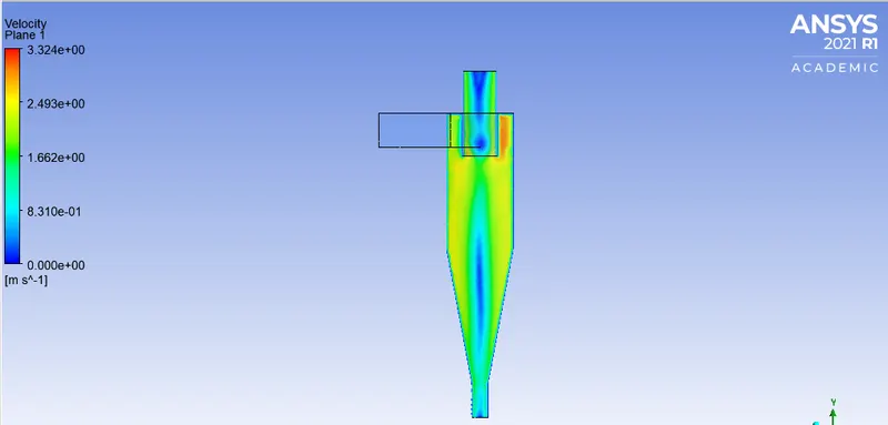
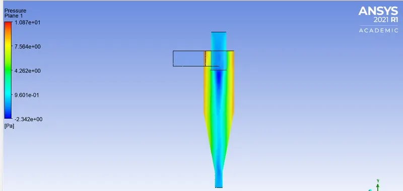
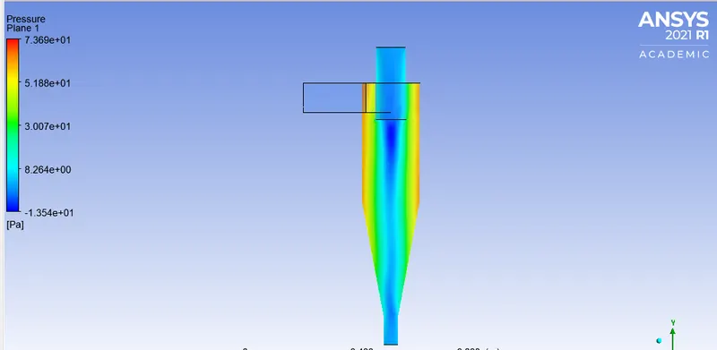
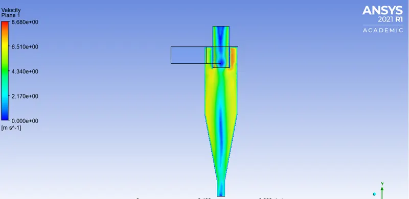
The pressure field has gradients in the radial direction, it decreases rapidly from the wall to the center of the axis. With an increase in velocity the pressure drop increases. The flow field in the cyclone indicates the expected forced/free combination of the Rankine type vortex. Moreover, because the cyclone has only one gas inlet, the axis of the vortex does not coincide with the axis of the geometry of cyclone. Tangential velocity is the most dominant of all velocities, it is zero in the wall and the centre. The velocity decrease as we go down, and forms a chaotic flow around the upper mid section. Sometimes problems of flow reversal also occurs due to which, there is a lot energy loss, also called flow short circuiting.

The diameter of upward flow is slightly larger than that of the vortex finder. Moreover, since much gas flows over into the vortex finder, the axial velocity reaches a peak value under the vortex finder. Meanwhile, the dip in axial velocity near the axis except the section under the vortex finder is clearly visible. The center of the flow does not coincide with the geometric centre, hence eccentric vortex finders are required.

Since the axis of the forced vortex is not coincident with the geometric axis of cyclone distribution of radial velocity is eccentric, the improper structure maybe due to gas extrusion. There is lot of secondary recirulation regions caused due to collision of radial and axial flows, eddy flows, flow short-circuiting and reversals due to particulate friction generate these secondary regions.

Factors that effect separation efficiencies are particle positions in the inlet, ones entering from the top part having higher desent angles have better separation. Particles exceeding the size due to force balance from the wall, gas drag, gravity and centrifuge action tend to balance out and hece the particle collects.

Various geometric factors like cone length, body length, ratio of inlet port to diameter, cut-off diamter, collection efficiency etc.

MATHEMATICAL MODELS:

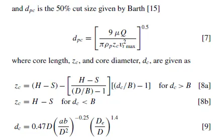
Iozia and Leith Model

This is model derived out of Barth & Model, it assumes that particle carried by the vortex is under influence of two forces centrifugal and flow resistance.

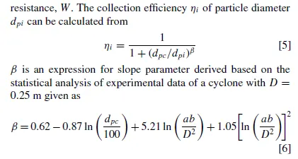
The cut-off diameter of Dpc is given by:

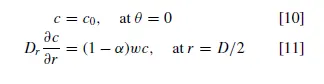
Li and Wang Model:

This model includes particle bounce or re-entrainment and turbulent diffusion in the wall, two dimensional analytical expression for particle distribution is hence obtained. Certain assumptions are made for the radial velocity i.e the distribution is not constant & boundary conditions are mentioned below:

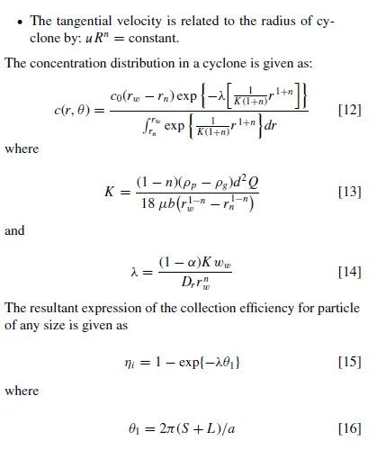
Koch and Licht Model

This model recognize the turbulent nature of cylones and distribution of gas residence times within the cyclone. Here the assumptions are tangential velocity of the particle is equal to that of gas flow & radius of cyclone depends on the tangential velocity.

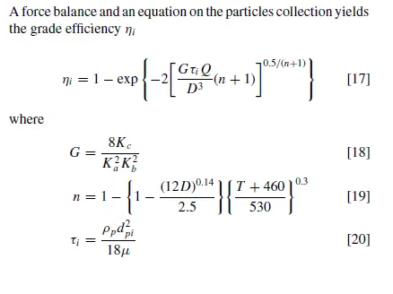
Tou is the relaxation factor, G is factor related to the cyclone and n to the vortex.

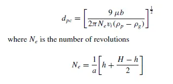
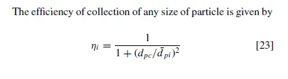
Lapple Model

It is a model that is based on force balance and influence of factors namely centrifugal and flow resistance, it assumes the particle is distributed evenly at the inlet. The collection efficiency is 0.5 from inlet to wall of cyclone, the cut-off diameters are computed as :

SIMULATION PREPERATION & MESHING

1. We import the geometry file in Spaceclaim, where we perform general geometry inspection, then proceed towards preperation.

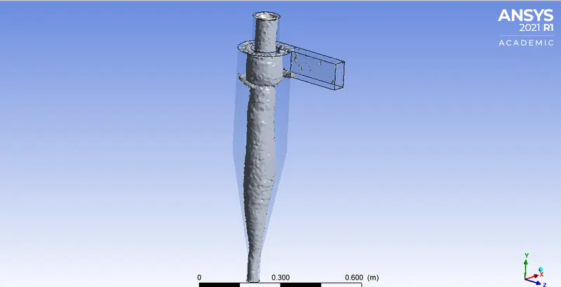
2. We perform volume extraction, ensure clicking the inner edges of the volume, or else we may encounter meshing error.

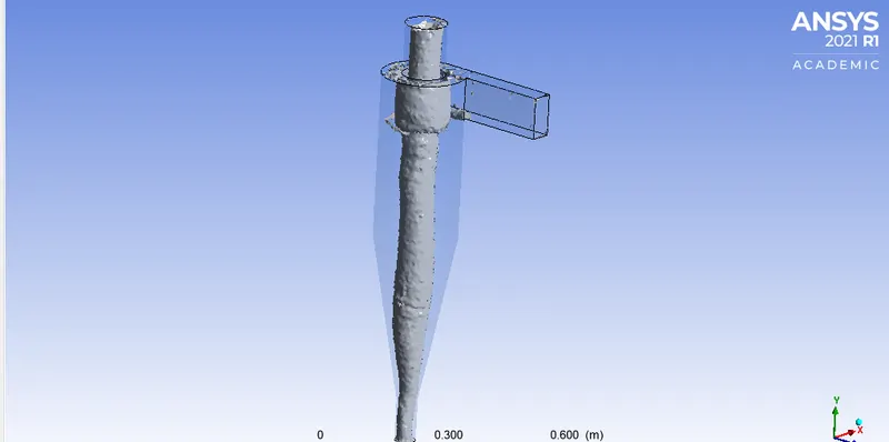
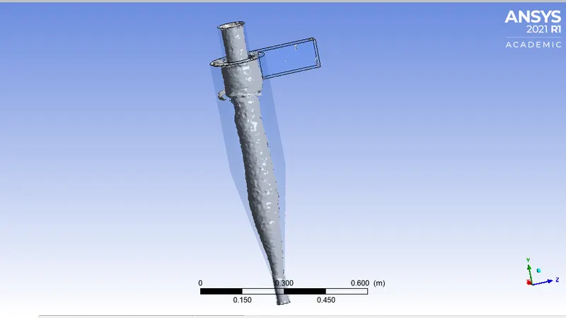
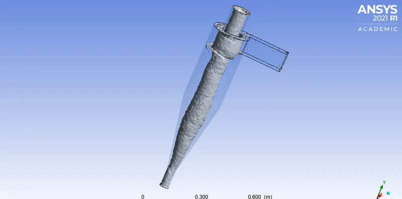
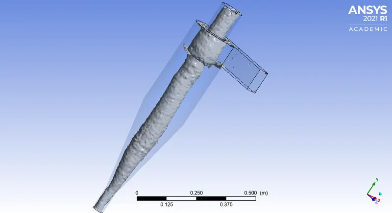
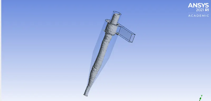
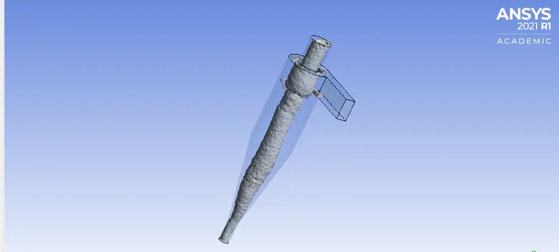
The volume post extraction looks like this:

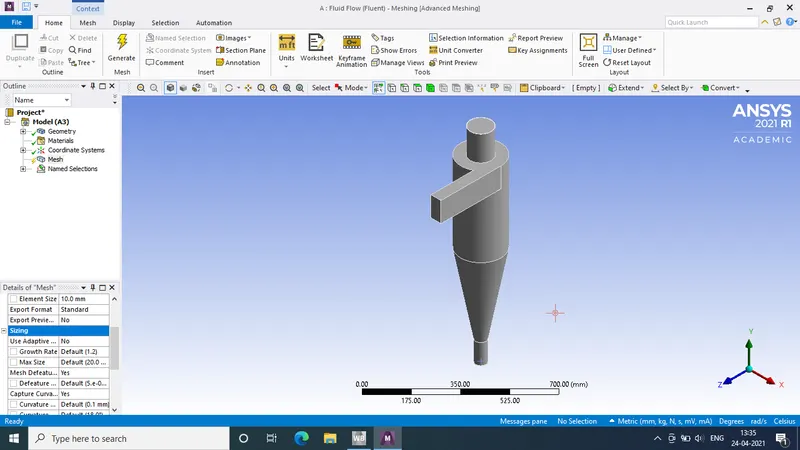
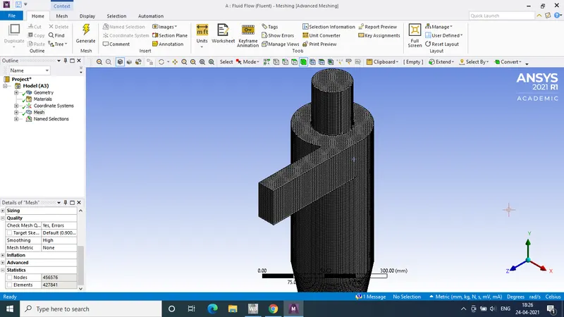
We proceed towards meshing:

1. Setting the global mesh to 10mm

2. Capture curvature turned-on

3. Smoothning-High

4. Body mesh-5mm

5. Mark named selections- Inlet, outlet1&2.

Elements-427841, Nodes-456576

The mesh looks like this:

SETUP IN FLUENT

Its important we know that we would be simulating 10 cases, The first 5 with different dia from ( 1micro-5micro) with 3m/s named as case a,b,c,d,e. Other cases are named 1,2,3,4,5 with same dia ( 5 micro), different velocity from (1-5).

1. We perform a steady state simulation, with gravity enabled in negative y-direction.

2. Select RNG model, with swirl dominated option.

3. To enable DPM( Discreet phase modelling):

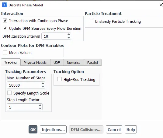
Enable the options shown above, important to note to have a complete simulation, we increase the Max. number of steps to 150000.

4. We then proceed towards injection settings:

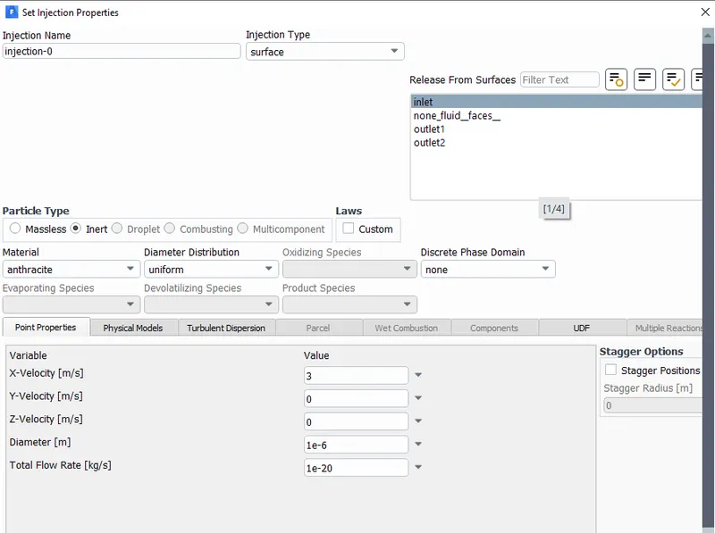
Vary the x-velocity & diameter of the particle according to the case. Choose surface injection from the inlet and keep the total flow rate as default, also name the injection in accordance.

5. Proceed towards boundary condition settings:

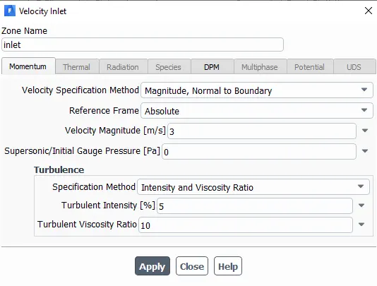
Change parameters accordingly

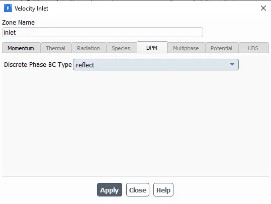
Boundary DPM settings followed for our simulation:

Inlet and wall:- Reflect

Outlet(Top):- Escape

Outlet(Bottom/dustbin) - Trap.

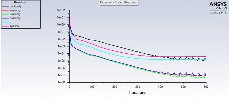
6. Uncheck the convergence criterion

7. Set the methods to second order upwind, pressure velocity coupling as SIMPLE.

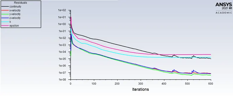
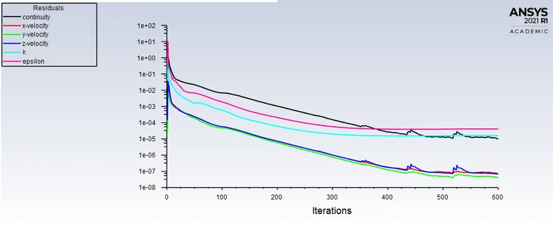
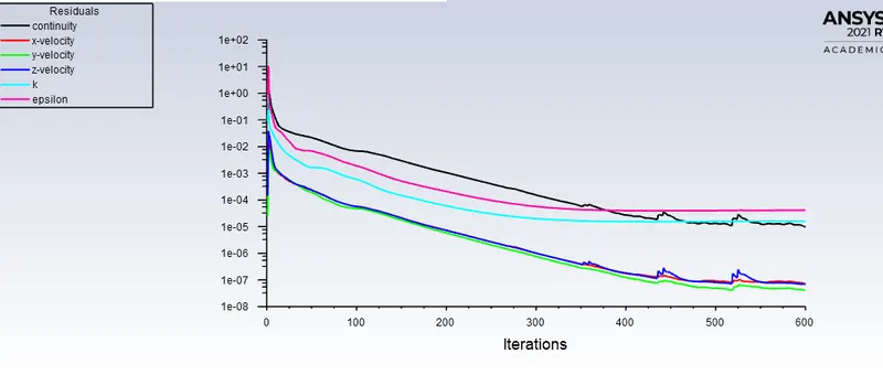
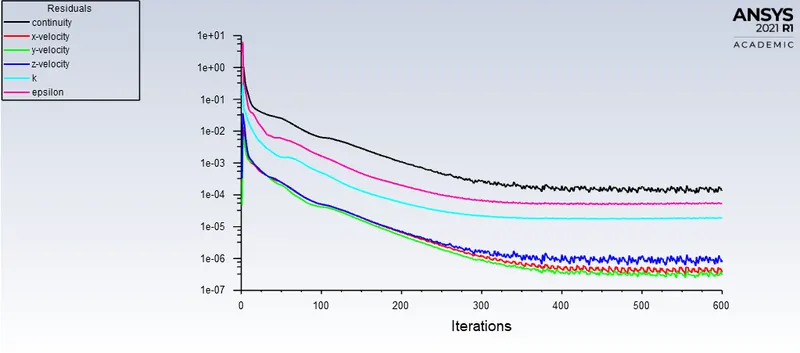
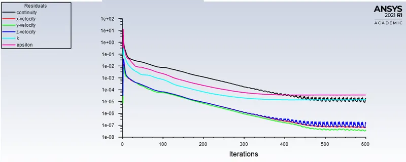
8. Standard initialize, from the inet & run it for 600 iterations.

RESULTS & CONLUSION:

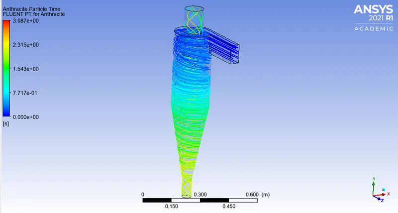
Case-a

Case-b

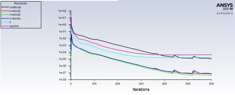
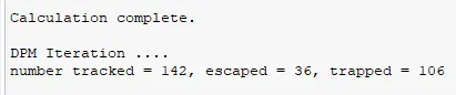
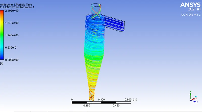
Case-c

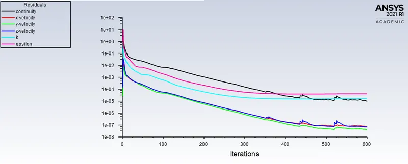
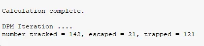
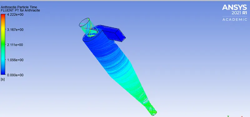
Case-d

Case-e

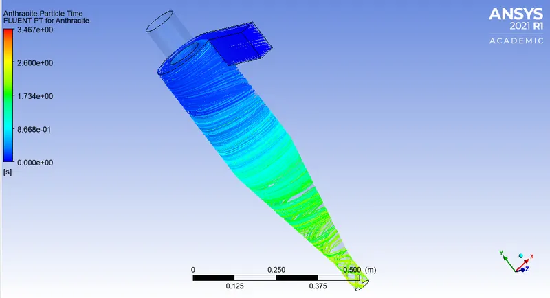
Pressure plots, velocity plots and differential:

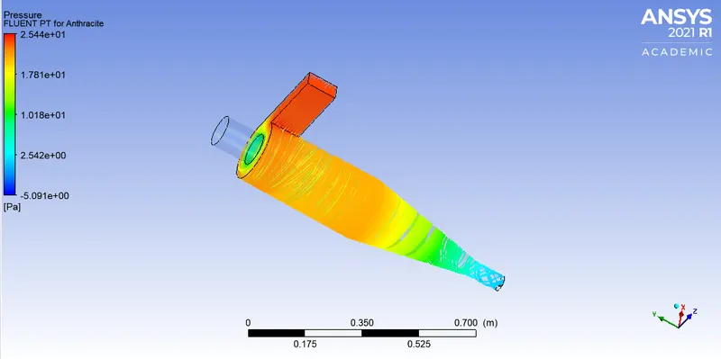
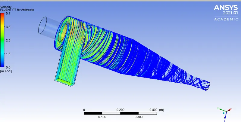
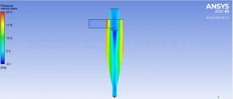
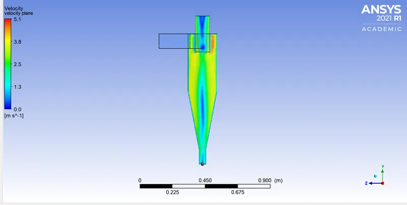
Pressure differential for this case (3m/s)= 24.0798-(-0.0100944)

= 24.0898944 Pa

Case-1 (1m/s)

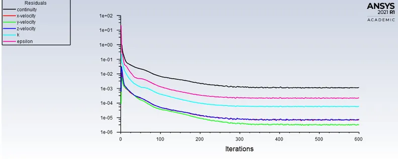
Inlet pressure-curve:

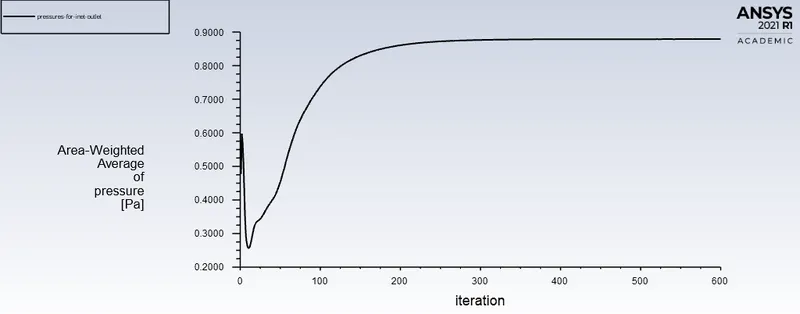
Pressure differential for this case (1m/s), (Inlet-outlet1)= 2.252-(-0.00359)

= 2.25559 Pa

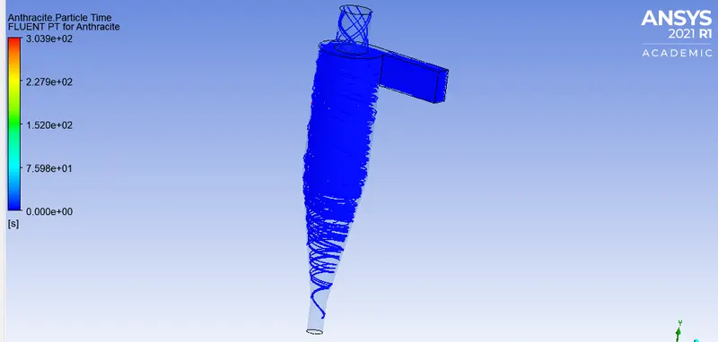
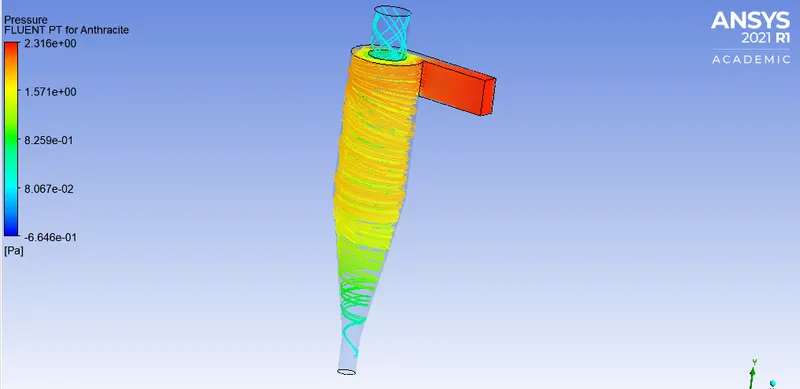
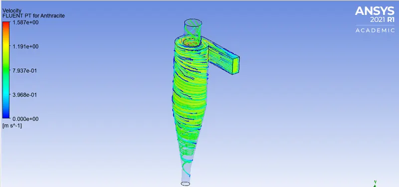
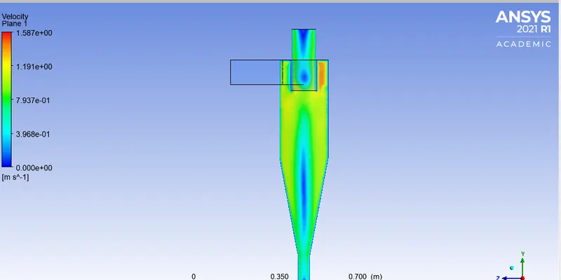
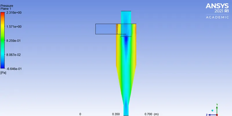
Case-2 (2m/s)

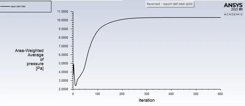
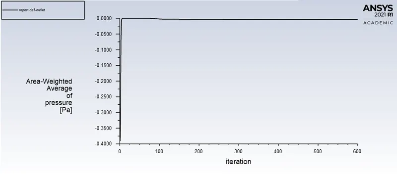
Pressure differential for this case (2m/s), (Inlet-outlet1)= 10.319-(-0.003621)

= 10.322621 Pa

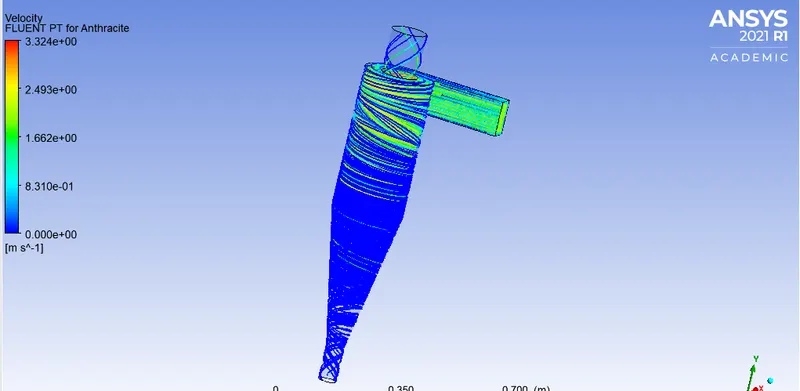
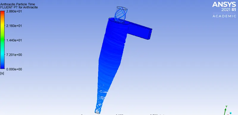
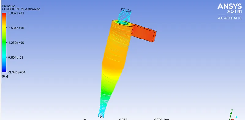
Case-3 (4m/s)

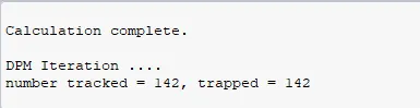
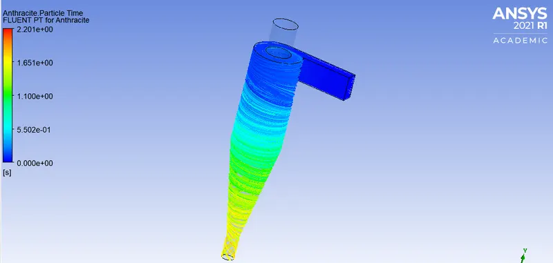
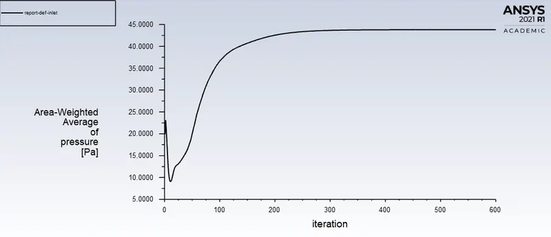
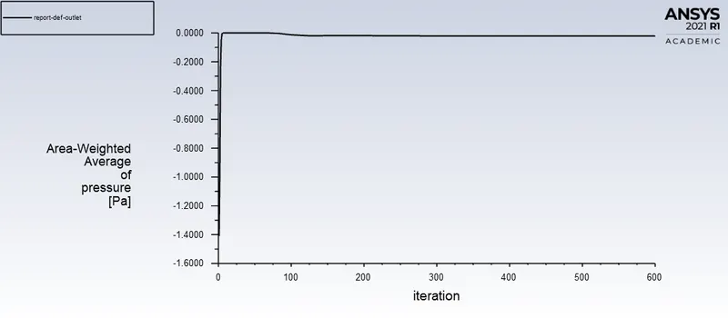
Pressure differential for this case (4m/s),(Inlet-outlet1)= 43.80-(-0.0208055)

= 43.108805 Pa

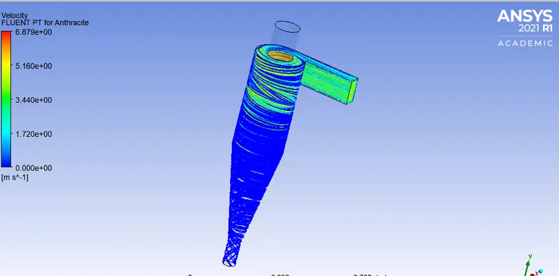
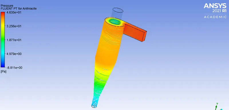
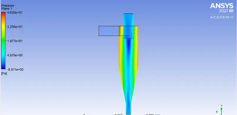
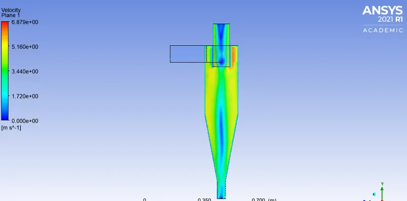
Case-4 (5m/s)

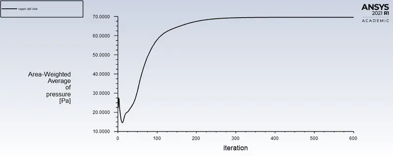
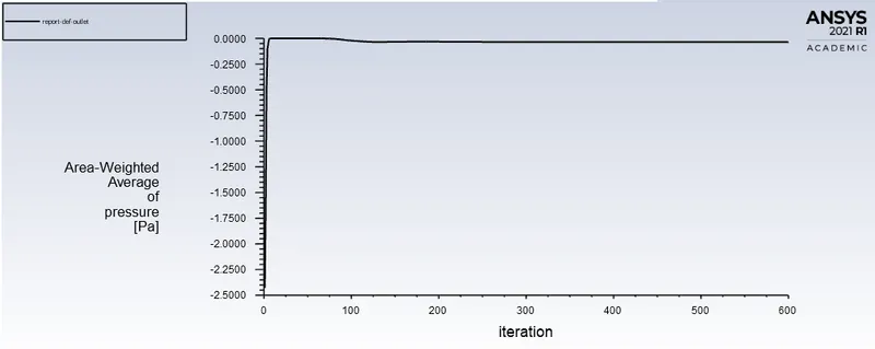
Pressure differential for this case (5m/s), (Inlet-outlet1)= 69.571-(-0.03595)

= 69.60695 Pa

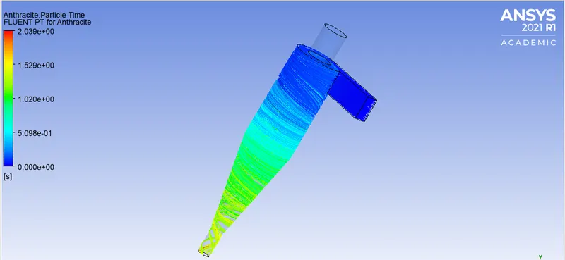
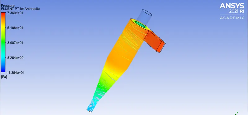
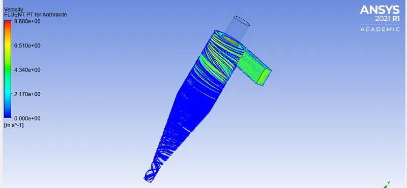
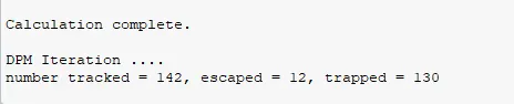
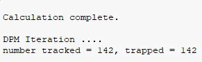
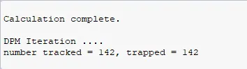
Case 5 micro meter, 3m/s was not simulated as it has been done already earlier. An important factor indicating seperation efficiency of the seperator is trapped particle/tracked particle ratio, which is calculated for every case.

CASES	SEPRATION EFFICIENCY	VELOCITY (m/s)	Pressure difference (Pa)	DIAMETER (micro meter)
a	69.7% (99/142)	3	24.08977	1
b	74.6% (106/142)	3	24.08977	2
c	85.21% (121/142)	3	24.08977	3
d	91.54% (131/142)	3	24.08977	4
e	100% (142/142)	3	24.08977	5
1	<7% (NA/142)	1	2.252359	5
2	21.81% (31/142)	2	10.322621	5
3	100% (142/142)	4	43.108805	5
4	100% (142/142)	5	69.60695	5

CONCLUSIONS:

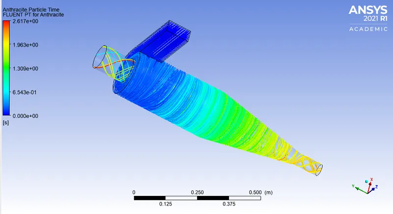
1. The plots and contours match well with existing literature, the structure of the vortex, the residence time, velocity & pressure mid-planes.

2. As the diameter and the tangential velocity of the cyclone seperator increases the seperation efficiency also increases

3. There is an increase in pressure drop as the velocity increases, so we can higher pressure drop better the seperation efficiency.

4. The reason why the standard k-epsilon and Realizable k-epsilon models were not used as they were not optimized for the strongly swirling flows typically found in cyclones. The RNG k-episilon model can be
used with about 12% deviation on experimental data. This model underestimates the variation of the axial velocity profile across the radial direction and also overestimates the magnitude of the tangential velocity and the cyclone pressure drop.

5. For very low inlet velocities i.e below 2m/s the seperation process is highly inefficeint.The same goes for diameters lesser than 3 micro meter.