Week 4 - CHT Analysis on Exhaust port

OBJECTIVE OF SIMULATION:

1. To set up CHT(Conjugate heat transfer) simulation

2. To show the temperature distributions and velocity profile for the exhaust port.

3.To verify the simulation with theory.

4. We would simulate using k-epsilon and k-omega SST models.

THEORY:

Heat, according to thermodynamics is a form of energy in transit hence CHT can be inferred as the transfer of heat from one interface to another. In our simulation, we are concerned with a solid-fluid interface. Heat transfer occurs due to temperature gradients. In most, engineering applications the solid is immersed in the fluid, or the fluid is made to move within the solid boundaries, in our case, it's the latter.

There are two main dominant modes of heat transfer for our problem, Conduction, and Convection.

Conduction is a heat transfer method dominant in a solid-solid interface, where energy is transferred by virtue of increased oscillations of atoms about their mean position, and they collide with the neighboring ones.

, is the general formula for conduction, dell T is the temperature gradient and k is material conductivity.

Convective heat transfer is usually seen in a solid-fluid interface, where fluid and solid molecules interact and facilitate heat transfer. , where h is the convective heat transfer constant, A is the area, dell T is temp difference.

The thing to note is Conduction depends on heat variation w.r.t spatial distance, whereas, Convection depends on the temperature difference between Solid- fluid interface.

Convection is a bulk phenomenon, where the molecules with receive or transfer energy, owing to changes in density, form a convective cycle.

CHT is crucial in various heat exchanging devices, like coolers, heaters where the process of heat transfer, has to be made feasible and efficient. Sometimes additives are added to the fluid media to enhance heat transfer. In the automobile industry, the cooling performance of water jackets can be improved to increase the shelf life of the engine. Apart from efficient cooling or heating, it's important for designers to look out for regions where temperatures are high to look out for thermal stresses. This increases the service time of the component.

In our case the convective heat transfer is dominant, the conductive transfer can be seen in the solid volume of the exhaust port.

SIMULATION SET-UP

We begin the simulation set-up, by importing the model in space-claim

Things to note:

1. To repair the edges if unable to select edges.

2. Extract the fluid volume. ( Use edge select)

3. Distinctly mark the volumes as solid and fluid.

4. Go to the workbench to enable sharing topology option. ( To have conformal mesh)

The prepared geometry would have pink circles:

The mesh set-up can be achieved as follows:

1. The first step would be to create all named selections, inlets, outlets, the solid boundaries can be written as outer-wall with the convective transfer condition. The inner part after hiding the body can be written as inflation layers. The unselected walls are given an adiabatic condition. The dominant cell is tetrahedral.

2. The inflation layers can be set up, from the inflation option, choosing the req named selection, with total thickness, set as 3mm, with 5 layers.

3. It's important to select capture curvature, and the element sizing can be bought to 18mm.

The nodes- 142768, elements-428879.

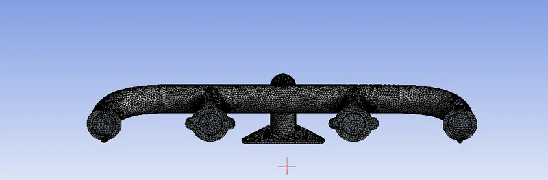
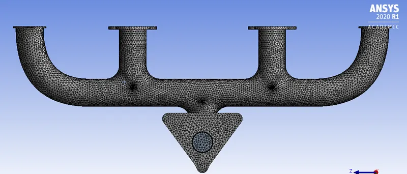
Inflation layers:

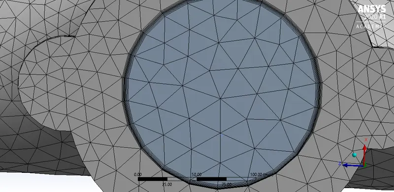
The mesh metric:

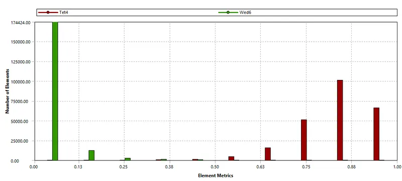
SET-UP IN FLUENT

The set-up in fluent can be done as:

1. Pressure- base solver, Steady-state.

2. Models- Case-I ( k-epsilon), Case-II ( k-omega), Energy equation turned on.

3. Materials- Solid is aluminum, fluid is air with standard properties.

4. Boundary Conditions- Inlet-5m/s and thermal- 700K.

Outlet- 0 gauge.

Wall conditions- Heat transfer coefficient for convective wall- 20 W/mC*

For all other walls, heat flux is zero.

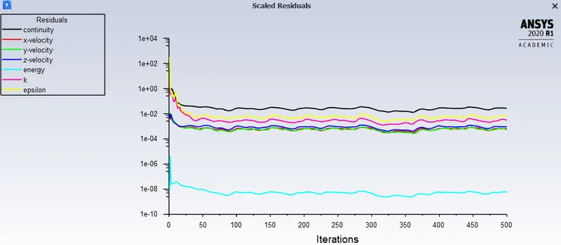
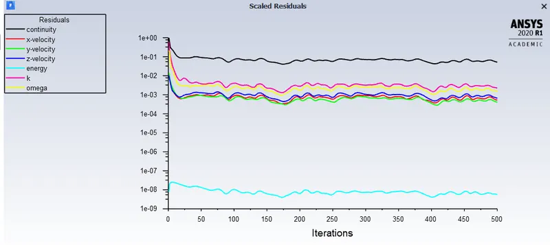
5.Residuals checked for convergence.

6. Hybrid Initialized.

The calculation set-up for 500 iterations.

The plots, streamlines can be seen in CFD-Post.

RESULTS

CASE-I

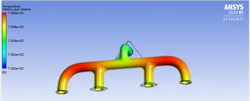
Temprature distribution:

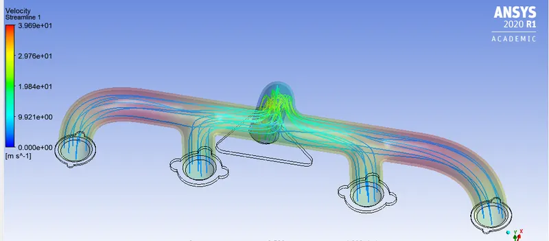
Streamlines velocity:

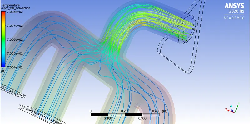
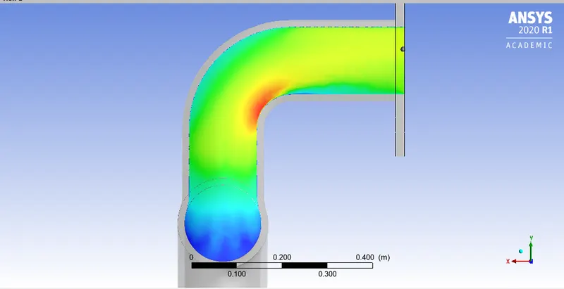
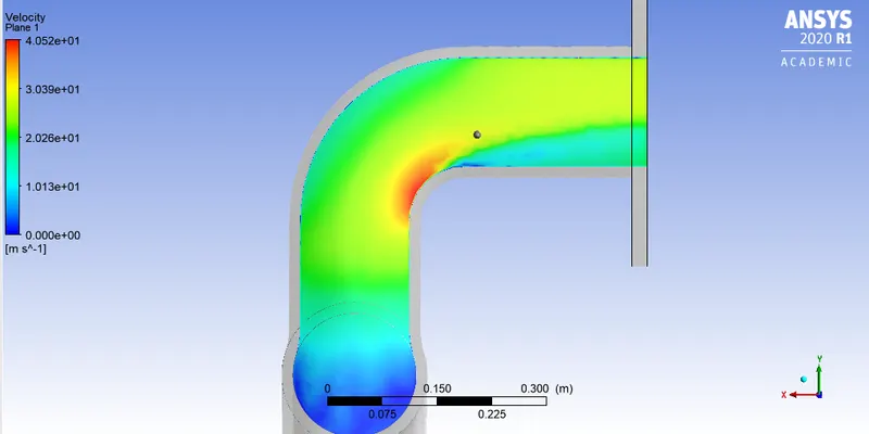
Velocity at outlet curve:

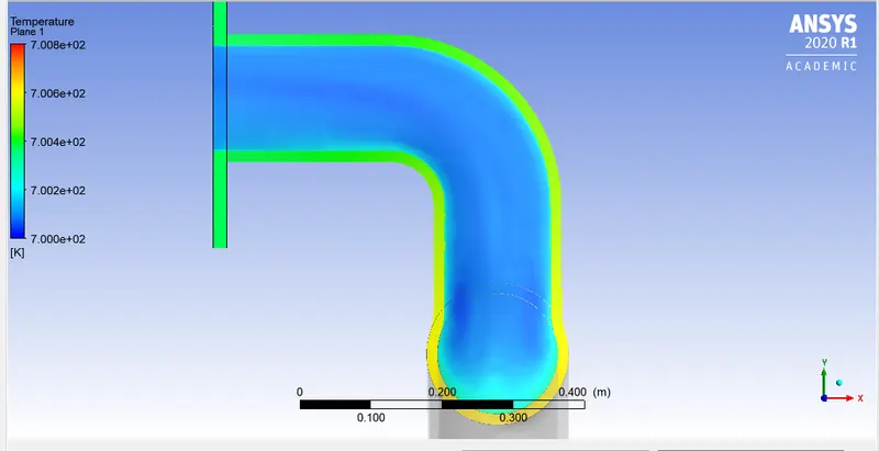
Temperature at the outlet curve:

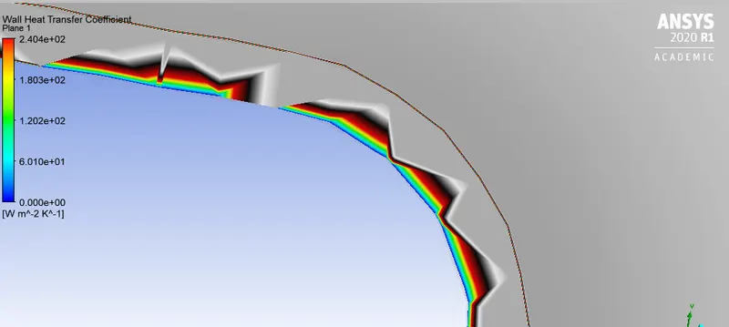
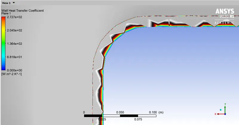
Heat transfer coefficient:

CASE-II

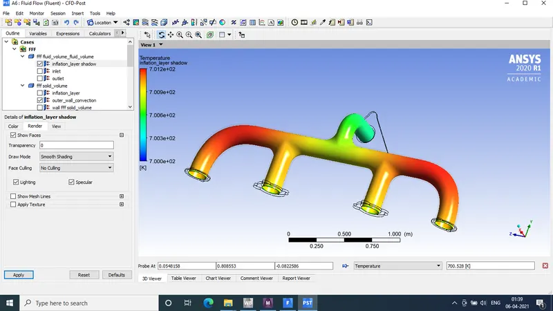
Temprature distribution:

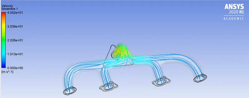
Streamlines:

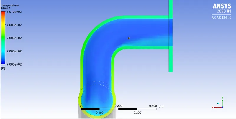
Temprature at outlet:

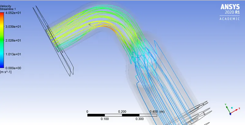
Velocity at outlet:

Heat transfer coefficient:

DISCUSSIONS AND RESULTS:

1. On observing the residuals the velocity and continuity show divergence, even after convergence.

2. We see the temperature is high at the bends, the reason being mass conservation we know the areas of inlets are all same since there is a single outlet only, the fluid mass in-order to be conserved, increase the velocity, we see the red patch in the velocity contours.

3. The Nusselt number is Nu=0.023Re^4/5*D*Pr^n, where Pr is Prandtl number, Re is Reynolds number since Re is proportional to velocity, the CHT depends on velocity, this is in coherence with the results we can max heat transfer at the bend, where the velocity is maximum at the outlet.

4. The mesh size, inflation layers, and conformal mapping are necessary for good results.

5. SST-omega is a better model, it's more in coherence with the theory, better-developed velocity profiles can be observed, and since the wall functions capture the boundary interactions much better.