Week 1: Channel flow simulation using CONVERGE CFD

OBJECTIVE OF THE SIMULATION:

1. To simulate flow along a rectangular channel.

2. To simulate with three grid sizes.

3. To understand the flow parameters and their variations.

THEORY:

Pipe flow or channel flow is one of the most widely seen flow situations in a plethora of applications ranging from engineering, domestic, industrial, and academic applications. Owing to its wide range of applications, it naturally becomes a center of study to better understand flow physics. Pipe or conduit flows are internal flows, their boundary conditions are different when compared with external flows and this must not be confused with open channel flows, as the boundary conditions vary.

There is no direct interaction of the atmosphere with the flow, but hydraulic forces are exerted on the channel body. By using predictive methods like CFD, we can estimate the flow losses (loss in velocity and pressure), compute structural stresses, understand mixing patterns, and have an idea about the flow structure.

Let's look at the channel flow in detail, pipe flow is generally governed by three forces viscous, inertial, and gravity forces. Now the Reynolds number plays a vital role in determining the nature of the flow.

In our case, we have considered laminar flow, hence we would be looking at the Hagen-Poiseuill Formula

The derivation of the formula and the dependence is shown below:

                              

                              

               

     

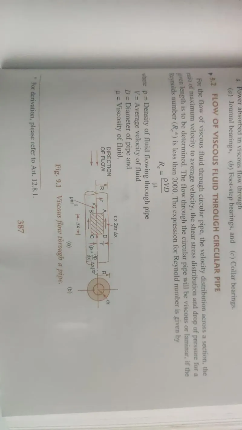
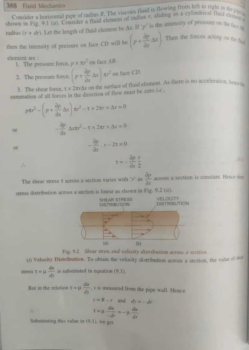
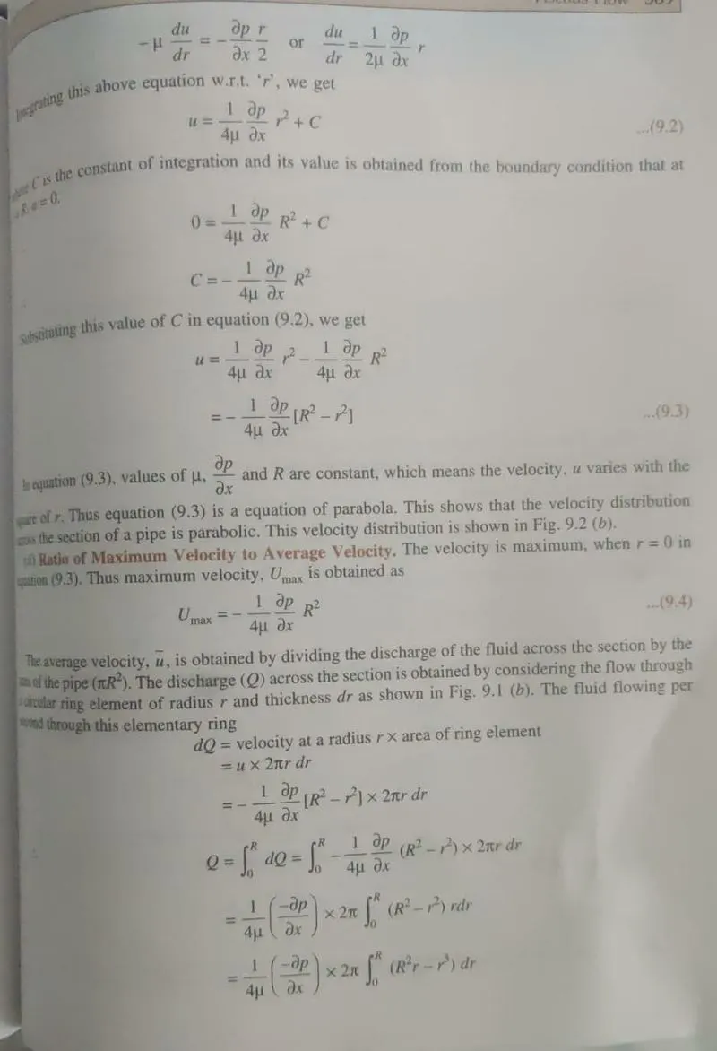
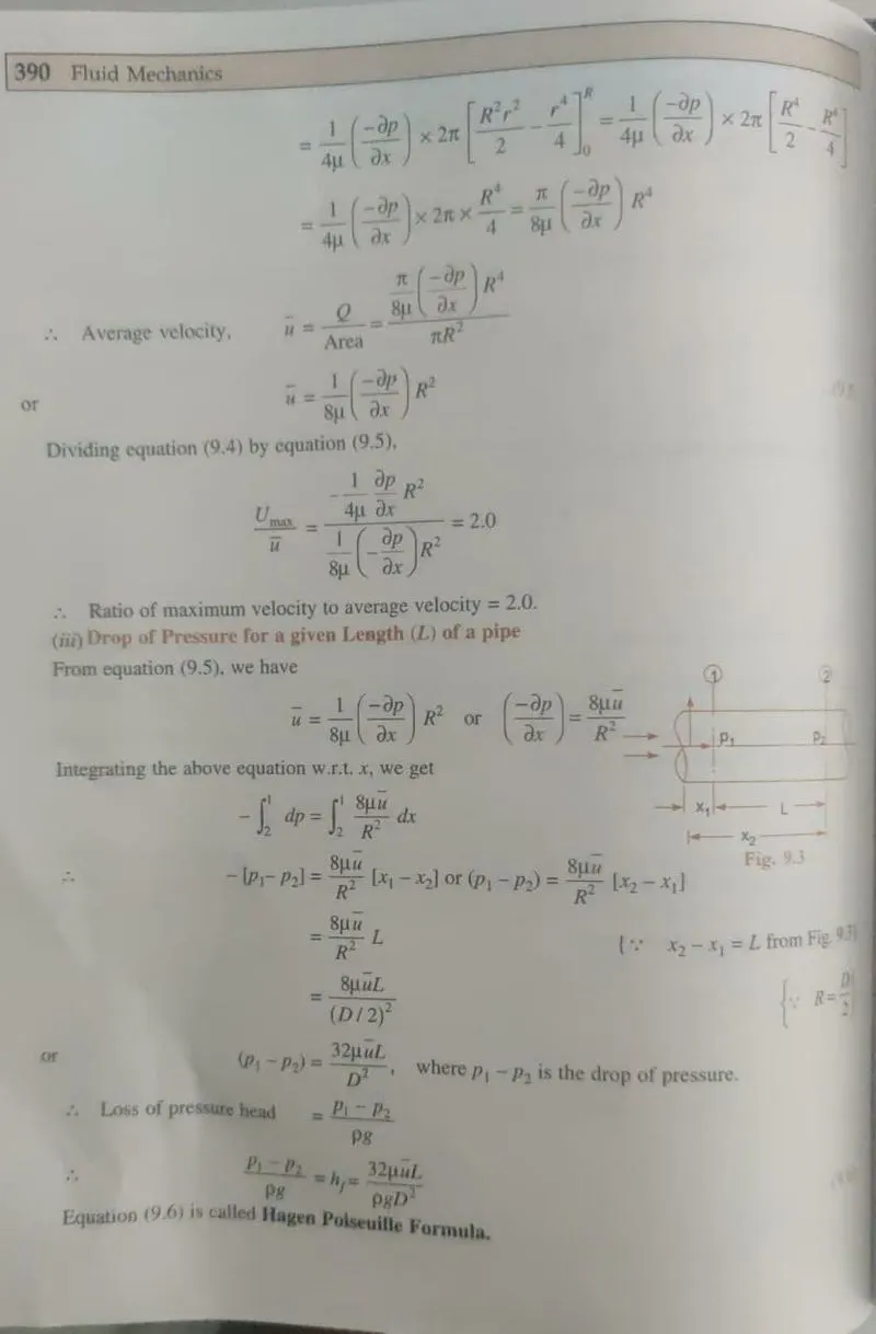
As we can see from the above derivation:

1. Shear stress depends on radial location and pressure gradient.

2. Velocity depends on radial location, pressure gradient, and viscosity of the fluid.

3. The pressure drop depends on characteristic length, viscosity, Diameter of the pipe, average velocity, and specific weight.

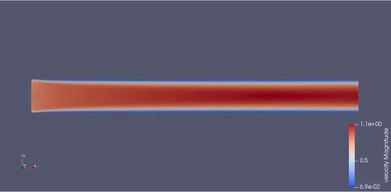
 Since the velocity equations are parabolic in nature, it will be maximum in the pipe centerline and minimum near the walls.

SETUP:

1. Pressure-based steady-state solver, in general, flow option, also keep the pre-defined mixture of air.

2. Define fluid region, with air and its correct mass fraction.

3. Assign boundaries with the inflow boundary at pressure 100001 Pa, and outlet as 100000 Pa.

4. Turn off all turbulence parameters.

5. In steady-state parameters set the range from 0-15000 cycles, keep all other parameters as 1e-9.

6. Ensure your CFL numbers are within the range of 0-1.

7. Correctly choose your time interval for writing text and 3-D files (1e-6).

RESULTS:

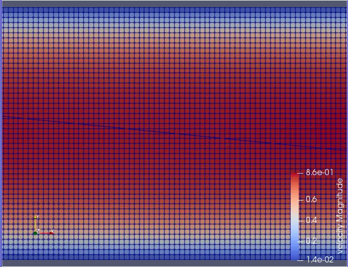
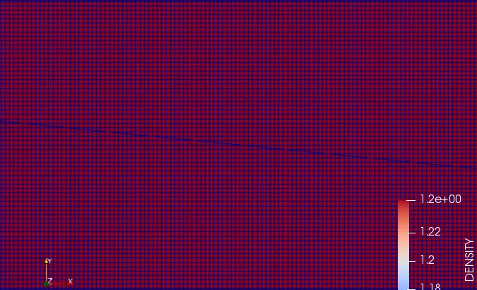
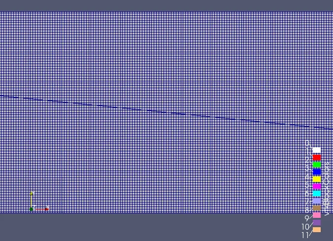
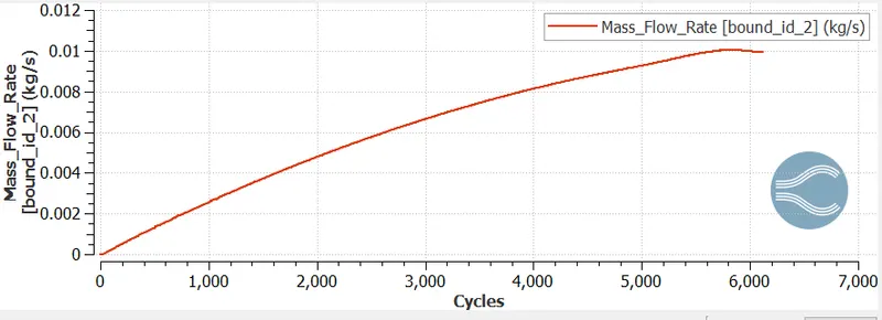
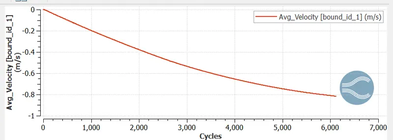
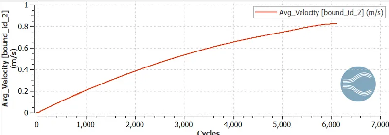
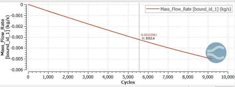
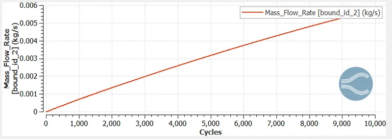
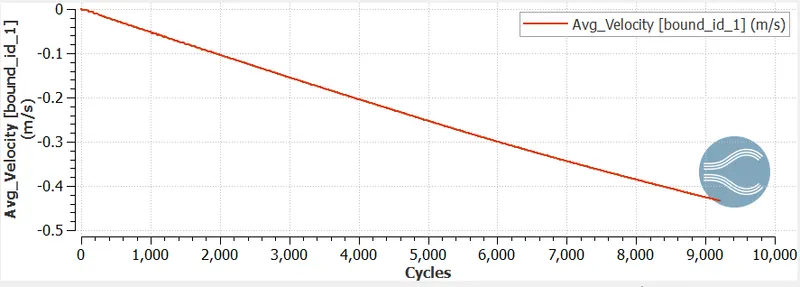
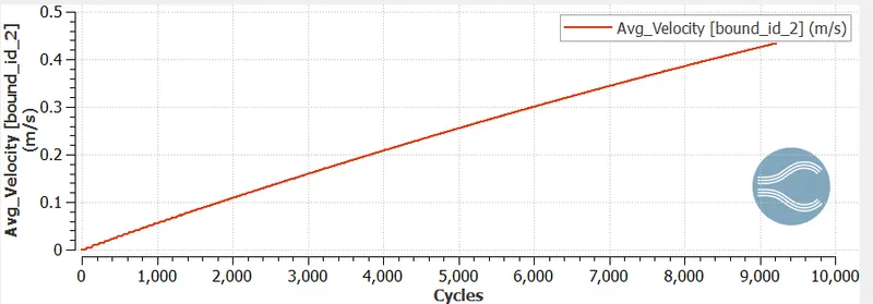
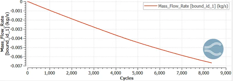
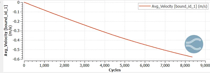
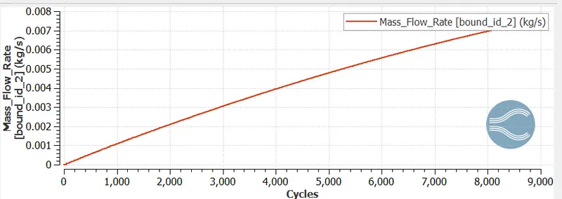
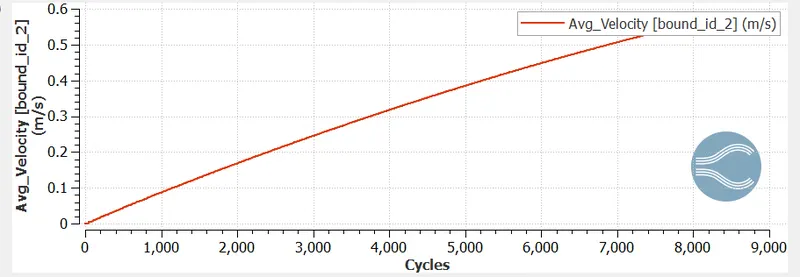
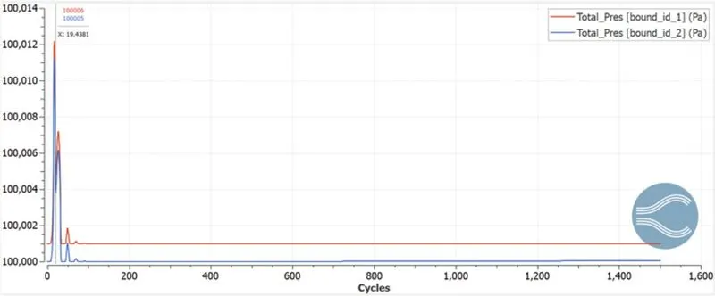
The results have been placed in case order of 1,2,3 (2e-4, 1.5e-4, 1.2e-4) The mesh sizes, velocity, pressure, density contours, and plots have been listed in order.

CASE-1 (2E-4)

 CASE-2 (1.5E-4)

 CASE-3 (1.2E-4)

 CASE-1 (2E-4)

CASE-2 (1.5E-4)

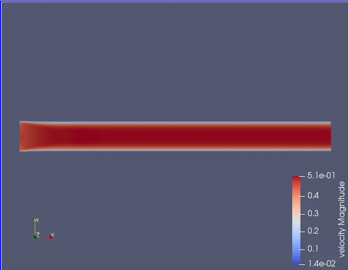
 CASE-3 (1.2E-4)

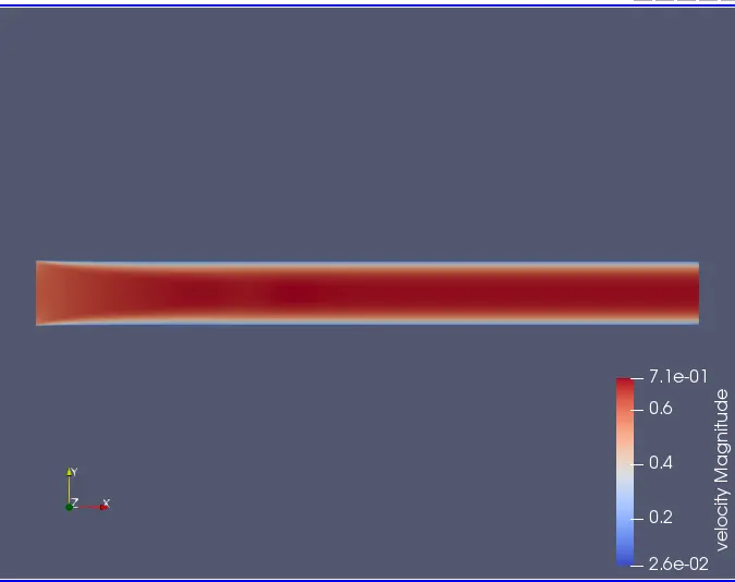
 CASE-1 (2E-4)

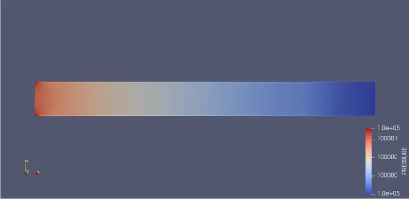
 CASE-2 (1.5E-4)

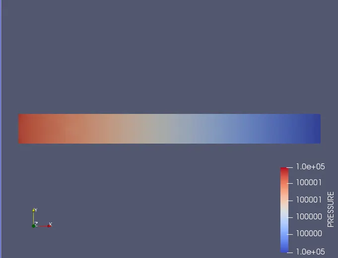
 CASE-3 (1.2E-4)

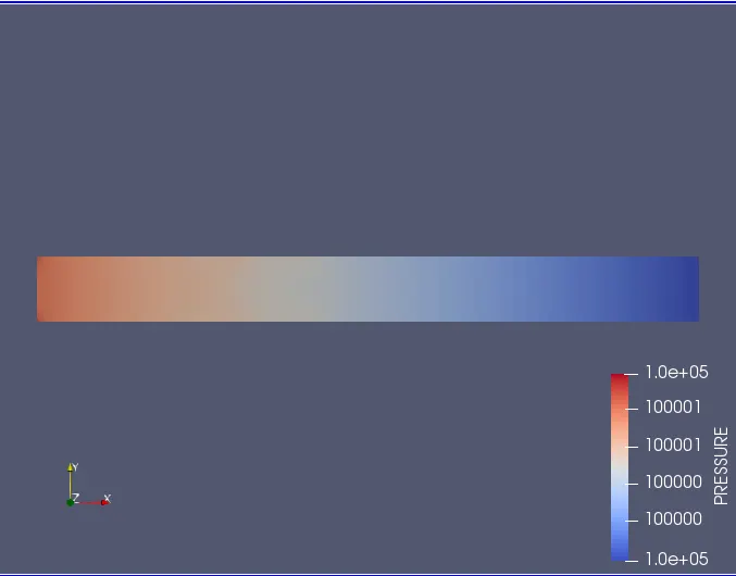
 CASE-1 (2E-4)

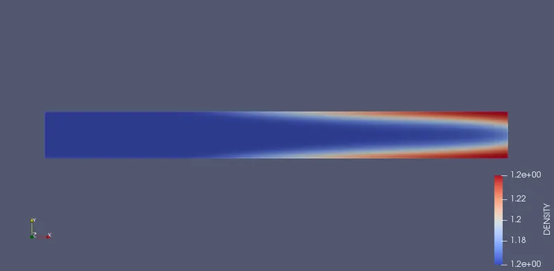
 CASE-3 (1.2E-4)

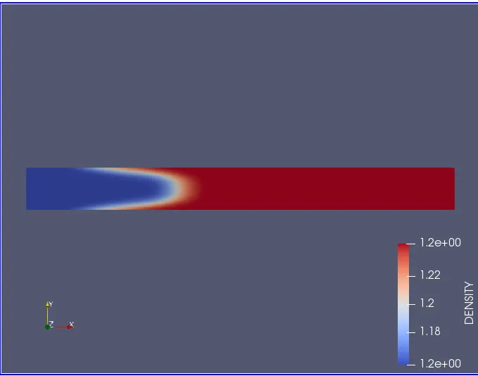
 CASE-1 (2E-4)

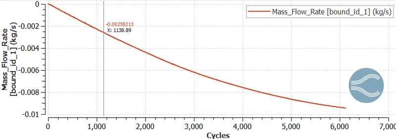
 CASE-2 (1.5E-4)

 CASE-3 (1.2E-4)

CONCLUSION:

1. The total pressure is a sum of static pressure and dynamic pressure, which almost remains constant slight losses can be seen at the output due to frictional and viscous losses.

2. The static pressure is slightly more at the inlet and lesser at the outlet as dynamic pressure is lesser at the inlet and more in the outlet, as energy is conserved along a streamline.

3. On reducing the grid size, we see more time taken for convergence as the number of cells where the governing equations are solved has increased.

4. The negative sign in the mass flow rate and velocity for the inlet indicates the flow direction along the channel.