Week 4.1: Project Steady state simulation of flow over a throttle body

Introduction

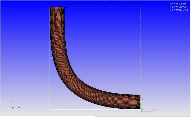
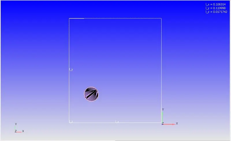
The Elbow contains a throttle which allows flow through it and helps in controlling the mass flow rate at the outlet. The purpose of this simulation is to understand the effects of introducing a thrtle and assessing its effects on the Velocity, Pressure and mass flow rate at the outlet. The Simulation is a Steady-state and runs tillthe solution converges. The geometry shows the elbow and the throttle.

Elbow

Throttle

Setup Configuration:

A steady state simulation is conducted with important configuration as follows:

Boundary:

Inlet	1.5e5 Pa
Outlet	1e5 Pa
Elbow wall	Law of wall
Throtle	Law of wall

Turbulance model:

K-Epsillon RNG

Grid:

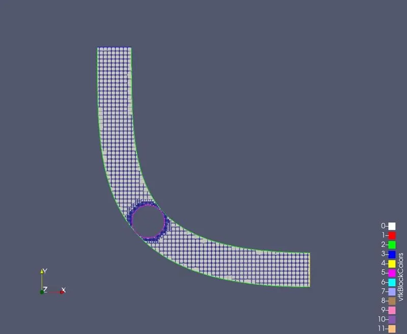
Size = 0.002 for all (dx, dy, dz) direction with fixed embedding at boundar: Throttle (Permenant)

Scale: 2

Embed layers: 3

Mesh:

Result

Plots:

Velocity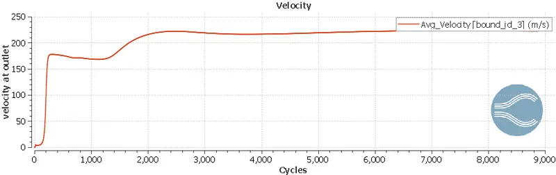
Mass Flow Rate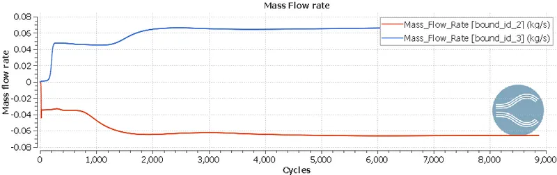
Total pressure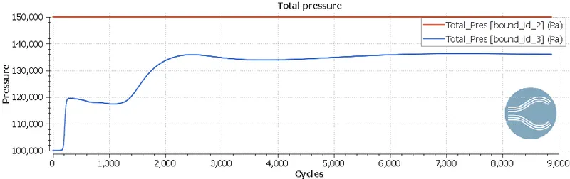
Cell count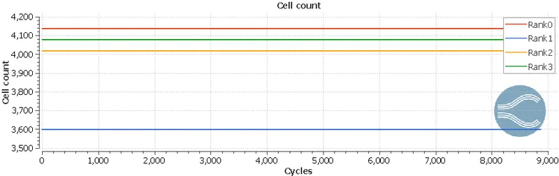

Contours:

Velocity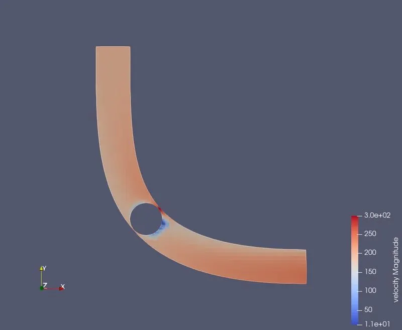
Pressure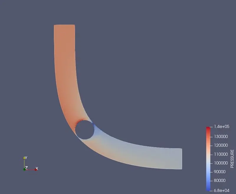

Animation:

Velocity

Pressure

Observation

It can be seen fro the results that the simulatio converges at about 9000th iteration/cycle. That means the properties such as mass-flow rate, pressue and velocites have stablised.

Also, by reading the output files and plotting them gives a good understanding of the si=olution has converges and since ther is not bolwing up or unnnatural oscillation in the outlet it can be concluded that the solution is close to accurate.

This simulation was run in parallel and the rank shows the distribution of the cells.