Week 3.5 - Deriving 4th order approximation of a 2nd order derivative using Taylor Table method

Theory: Taylor series approximation gives a pretty good approximation of a continuous function into an algebric form. It can give approximation of PDE of all forms and all orders. here we have an equation which is a second order derivative, `(del^2f)/(delx^2)`. According to Taylor series we can use 3 types of methods to approximate.

Central difference method: In this method we use symmetry, ie to compute a point's approximation we use a point ahead and behind (or) Top or bottom of point to compute for the point in question.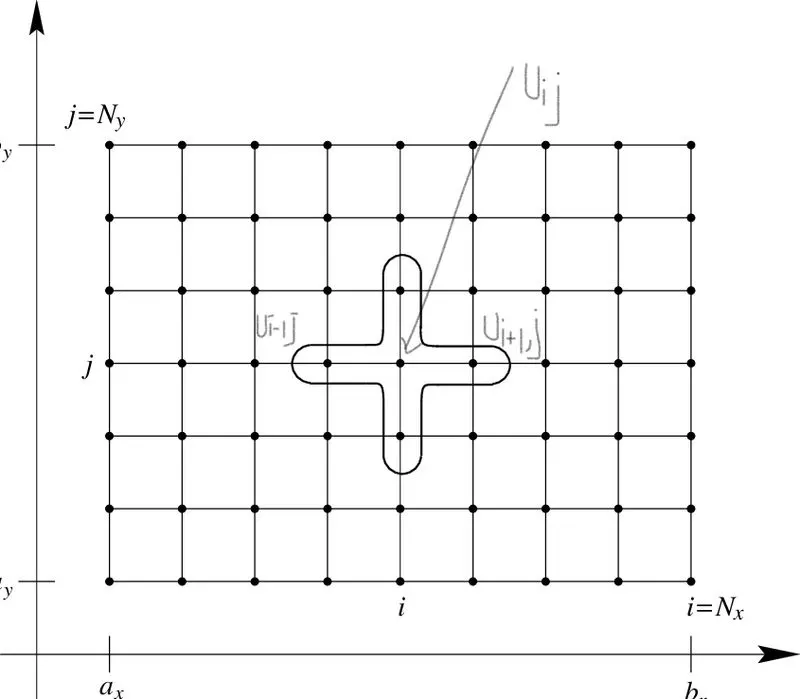

in this method information is gained by points surrounded by it.

2. Forward difference method/Right Skewed: In this type points ahead of the current points are used to compute the information about the current points. As given in the top right of photo.

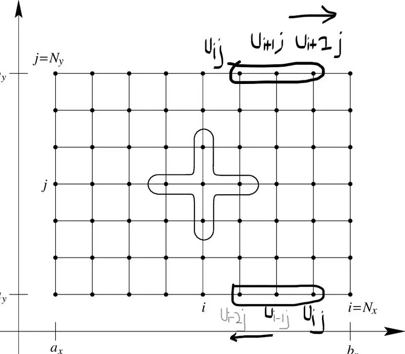
3.Backward/Rearward difference method/Left skewed:

This method uses points behind current point to compute it. As given in the bottom right of the photo.

To compute this Taylor table is used for the convinience. But to given the order of accuracy and the order of PDE the number of points will change. The number of points/ stencils we use 2 equations depending upon the desired outcome should be symmetic or skewed. The equations are given as:

i) The order of accuracy P = Number of nodes in the stencil N - order of derivative Q + 1 for symmetric/central schemes

ii) The order of accuracy P = Number of nodes in the stencil N - order of derivative Q for one-sided/skewed schemes

We use the first equation for central difference and second for the right and left skewed. With this we identify number of strensils as (5, 6) for central and Right/Left skewed respectively.

The general equations for all 3 methods:

Central method: `a*f(x-2*trianglex)+b*f(x-trianglex)+c*f(x)+d*f(x+trianglex)+e*f(x+2*trianglex)`

Forward difference method: `a*f(x)+b*f(x+trianglex)+c*f(x+2*trianglex)+d*f(x+3*trianglex)+e*f(x+4*trianglex)+f*f(x+5*trianglex)`

Rearward difference method: `a*f(x-5*trianglex)-b*f(x-4*trianglex)-c*f(x-3*trianglex)-d*f(x-2*trianglex)-e*f(x-*trianglex)-f*f(x)`

The derivation for the approximate equation for the 4th order approximation is given as (using Taylor's table):

1) Central Approximation method for a second order Function gives 5 stencils to work with. which is given into the table.

Sentncilsorder of approximation.	f(x)	`trianglex*f'(x)`	`trianglex^2*f^2(x)`	`trianglex^2*f^3(x)`	`trianglex^4*f^4(x)`
a(x-2dx)	a	-2*a	`a*(-2)^2/ (2!)*f^2(x)`	`a*(-2)^3/ (3!)*f^3(x)`	`a*(-2)^4/ (4!)*f^4(x)`
b(x-dx)	b	-1*b	`b*(-1)^2/ (2!)*f^2(x)`	`b*(-1)^3/ (3!)*f^3(x)`	`b*(-1)^4/ (4!)*f^4(x)`
c(x)	c	0	0	0	0
d(x+dx)	d	1*d	`d*(1)^2/ (2!)*f^2(x)`	`d*(1)^3/ (3!)*f^3(x)`	`d*(1)^4/ (4!)*f^4(x)`
e(x+2dx)	e	2*e	`e*(2)^2/ (2!)*f^2(x)`	`e*(2)^3/ (3!)*f^3(x)`	`e*(2)^4/ (4!)*f^4(x)`

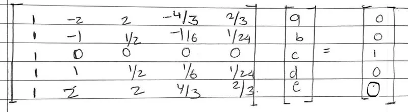
The values are a,b,c,d are calculated via matrix inversion,

As the give function is second order the `trianglex^2*f''(x)` will sum to 1 and the rest columns will be 0.

so, the given matrix obtained is:

`A*X = B`

2) Forward difference approximation/Right Skewed: The number of stencils for this is 6:

Sentncilsorder of approximation.	f(x)	`trianglex*f'(x)`	`trianglex^2*f^2(x)`	`trianglex^2*f^3(x)`	`trianglex^4*f^4(x)`	`trianglex^5*f^5(x)`
a(x)	a	0	0	0	0	0
b(x+dx)	b	`b*f'(x)`	`b*1^2/(2!)*f^2(x)`	`b*(1)^3/(3!)*f^3(x)`	`b*1^4/(4!)f^4(x)`	`b*(1)^5/ (5!)*f^5(x)`
c(x+2dx)	c	`2*c*f'(x)`	`c*2^2/(2!)*f^2(x)`	`c*(2)^3/(3!)*f^3(x)`	`c*2^4/(4!)f^4(x)`	`c*(2)^5/ (4!)*f^5(x)`
d(x+3dx)	d	`3*d*f'(x)`	`d*3^2/(2!)*f^2(x)`	`d*(3)^3/(3!)*f^3(x)`	`d*3^4/(4!)f^4(x)`	`d*(3)^5/ (5!)*f^5(x)`
e(x+4dx)	e	`4*e*f'(x)`	`e*4^2/(2!)*f^2(x)`	`e*(4)^3/(3!)*f^3(x)`	`e*4^4/(4!)f^4(x)`	`e*(4)^5/ (5!)*f^5(x)`
f(x+5dx)	f	`5*f*f'(x)`	`f*5^2/(2!)*f^2(x)`	`f*(5)^3/(3!)*f^3(x)`	`f*5^4/(4!)f^4(x)`	`f*(5)^5/ (5!)*f^5(x)`

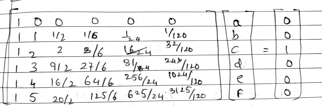
As the give function is second order the `trianglex^2*f''(x)` will sum to 1 and the rest columns will be 0.

so, the given matrix obtained is:

`A*X = B`

3) Rearward difference Method/ Left Skewed method: This method has same number of stensil but the values of a,b,c,d,e,f will be different than forward difference.

Sentncilsorder of approximation.	f(x)	`trianglex*f'(x)`	`trianglex^2*f^2(x)`	`trianglex^2*f^3(x)`	`trianglex^4*f^4(x)`	`trianglex^5*f^5(x)`
f(x)	f	0	0	0	0	0
e(x-dx)	e	`-1*e*f'(x)`	`b*(-1)^2/(2!)*f^2(x)`	`b*(-1)^3/(3!)*f^3(x)`	`b*(-1)^4/(4!)f^4(x)`	`b*(-1)^5/ (5!)*f^5(x)`
d(x-2dx)	d	`-2*d*f'(x)`	`c*(-2)^2/(2!)*f^2(x)`	`c*(-2)^3/(3!)*f^3(x)`	`c*(-2)^4/(4!)f^4(x)`	`c*(-2)^5/ (4!)*f^5(x)`
c(x-3dx)	c	`-3*c*f'(x)`	`d*(-3)^2/(2!)*f^2(x)`	`d*(-3)^3/(3!)*f^3(x)`	`d*(-3)^4/(4!)f^4(x)`	`d*(-3)^5/ (5!)*f^5(x)`
b(x-4dx)	b	`-4*b*f'(x)`	`e*(-4)^2/(2!)*f^2(x)`	`e*(-4)^3/(3!)*f^3(x)`	`e*(-4)^4/(4!)f^4(x)`	`e*(-4)^5/ (5!)*f^5(x)`
a(x-5dx)	a	`-5*f*f'(x)`	`f*(-5)^2/(2!)*f^2(x)`	`f*(-5)^3/(3!)*f^3(x)`	`f*(-5)^4/(4!)f^4(x)`	`f*(-5)^5/ (5!)*f^5(x)`

As the give function is second order the `trianglex^2*f''(x)` will sum to 1 and the rest columns will be 0.

so, the given matrix obtained is:

`A*X = B`

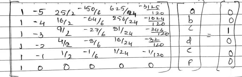
The solution for the a,b,c,d,e,f are directly routed to the code to compare the 3 methods.

Code below:

ploting and compilation of outputs from individual functions.

clear all 
close all
clc

%this script is puerly to plot the error comparision

%The following code compiles the output of function into an arrya.
%Considering the x=pi/3 and dx=pi/400

error = [central_approx(pi/3, pi/400), RightSkew(pi/3, pi/400), LeftSkew(pi/3, pi/400)];

%Plotting a bar graph.
bar(pi/400, error)

%The folloing plot will show the comparision as there is no output in
%commandline insted it is shown on the graph. Furthermore the legends and
%title is added using the tools availablwe in the plot itself.

Function for central difference approximation.

function error_1 = central_approx(x, dx)
%the following matrix is the result of Taylor table conversion of second
%order differential equation.

    A = [1 -2 2 -4/3 2/3;
        1 -1 1/2 -1/6 1/24;
        1 0 0 0 0;
        1 1 1/2 1/6 1/24;
        1 2 2 4/3 2/3];
    A_inv = inv(A);
    B = [0;0;1;0;0];
    sol = A_inv*B; %inversion of matrix method.

    analytical_solution = -2*exp(x)*sin(x); %analytical slolution of the given equation.
    
    %The central difference approximation for the given equation.
    %sol(i) is the result matix and substitutes a,b,c,d,e.
    central_approximation = sol(1)*(exp(x-(2*dx))*cos(x-(2*dx)))+sol(2)*((exp(x-dx))*cos(x-dx))+sol(3)*(exp(x)*cos(x))+sol(4)*((exp(x+dx))*cos(x+dx))+sol(5)*(exp(x+(2*dx))*cos(x+(2*dx)));
    
    %calculation of the error difference.
    error_1 = abs(analytical_solution - central_approximation);
end

Right skewed approximation:

function error_2 = RightSkew(x, dx)
%Same process follows here expect the matrix values.
    A = [1 0 0 0 0 0;
        1 1 1/2 1/6 1/24 1/120;
        1 2 2 8/6 16/24 32/120;
        1 3 9/2 27/6 71/24 (27*9)/120;
        1 4 16/2 64/6 (16*16)/6 (16*16*4)/6;
        1 5 25/2 125/6 625/24 (625*5)/120];
    A_inv = inv(A);
    B = [0;0;1;0;0;0];
    sol = A_inv*B;

    analytical_solution = -2*exp(x)*sin(x);
    
    %The given equation is right skewed.
    RightSkewed_approximation = sol(1)*((exp(x))*cos(x))+sol(2)*(exp(x+(2*dx))*cos(x+(2*dx)))+sol(3)*((exp(x+(3*dx)))*cos(x+(3*dx)))+sol(4)*(exp(x+(4*dx))*cos(x+(4*dx)))+sol(5)*(exp(x+(5*dx))*cos(x+(5*dx)));
    
    error_2 = abs(analytical_solution - RightSkewed_approximation);
end

Left skewed approximation:

function error_3 = LeftSkew(x, dx)
    A = [1 -5 25/2 -125/6 625/24 -(625*5)/120;
        1 -4 16/2 -64/6 (16*16)/6 -(16*16*4)/6;
        1 -3 9/2 -27/6 71/24 -(27*9)/120;
        1 -2 2 -8/6 16/24 -32/120;
        1 -1 1/2 -1/6 1/24 -1/120;
        1 0 0 0 0 0];
    A_inv = inv(A);
    B = [0;0;1;0;0;0];
    sol = A_inv*B;

    analytical_solution = -2*exp(x)*sin(x);
    
    %the given equation is left skewed.
    LeftSkewed_approximation = sol(5)*((exp(x))*cos(x))+sol(4)*(exp(x+(2*dx))*cos(x+(2*dx)))+sol(3)*((exp(x+(3*dx)))*cos(x+(3*dx)))+sol(2)*(exp(x+(4*dx))*cos(x+(4*dx)))+sol(1)*(exp(x+(5*dx))*cos(x+(5*dx)));
    
    error_3 = abs(analytical_solution - LeftSkewed_approximation);
end

Output:

Bar graph:

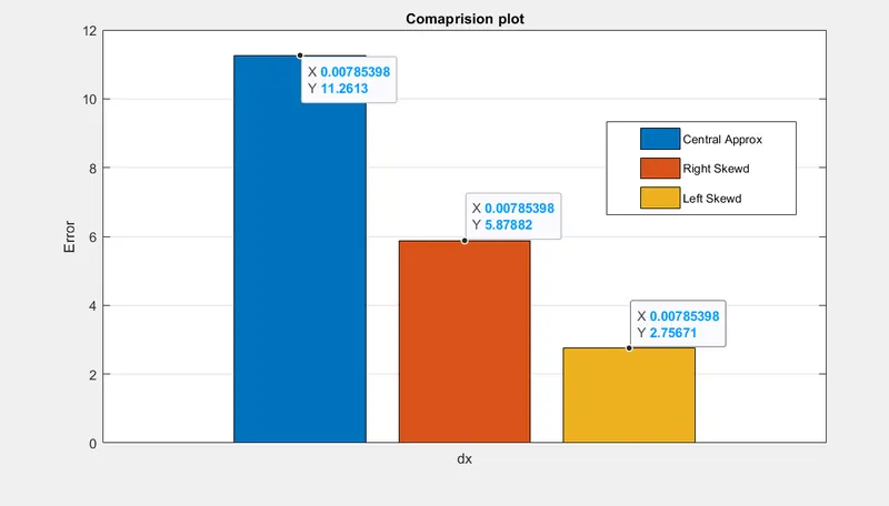
Comment on the graph and the viability of methods.

From primary observation it seems the central difference approximation isn't as accurate as right or left skewed. This seems like a reason enough to consider a skewed scheme than CD, But there is more to it. When we consider a problem statement, We often consider the boundary conditions, this can be a problem when we consider a CD becaude we g=have grid points on the surface and when we discrityze CD would seek points/node that are beyond the surface. This would be a problem and we wont get an accurate grid. In such cases using right, left skewed method helps by consider poins in only one direction. Also as evident from the graph it is accurate as well.