Week 3: Flow over a backward facing step
Aim: Flow over backwards facing step.
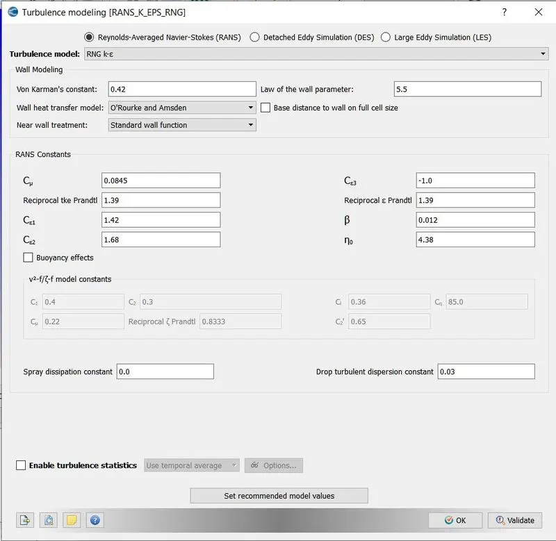
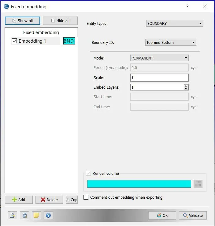
Introduction: backwards facing step is a crucila problem to test the code for CFD as it has lot of experimental data to check. In this simulation an attemp is made to understand the effects of finer grid and also to understand Flow separation. The geometry used is displayed as following. A turbulence model of K-Epsilon (RNG) is used. To fine tune the grid Fixed Embedding is used.
The 3 grid sizes used are as follows.
| Case 1 | 2e-3 |
| Case 2 | 1.5e-3 |
| Case 3 | 1e-3 |
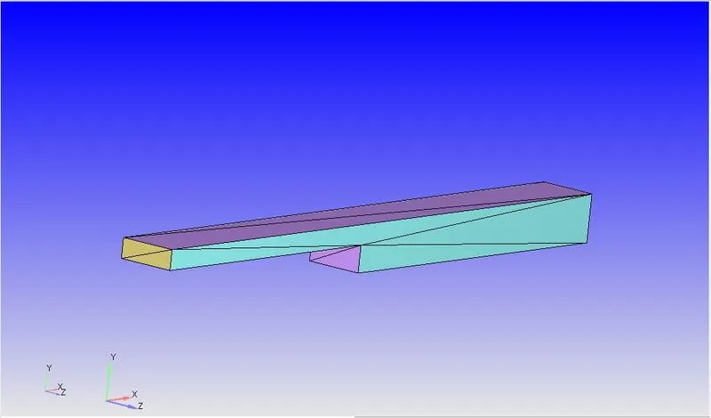 |
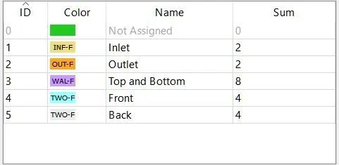
Boundary Flagging
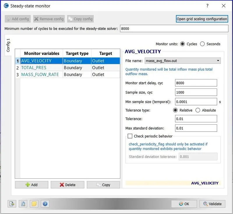
Steady state monitor (Monitoring for velocity, Pressure and mass flow rate)
Turbulence model (K-Epsilon rng)
Grid controls (Fixed embedding)
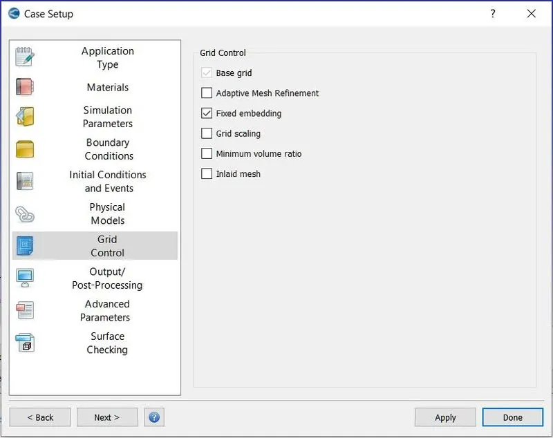
Fixed Embedding.
Simulation results:
| Case 1 | |
| Velocity | 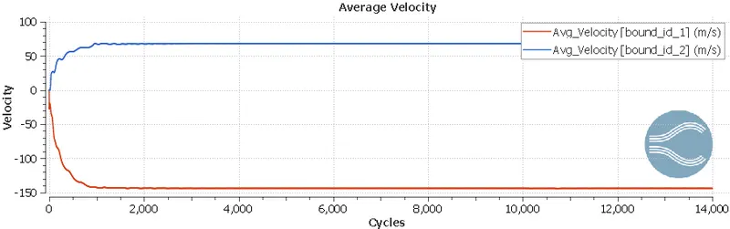 |
| Pressure | 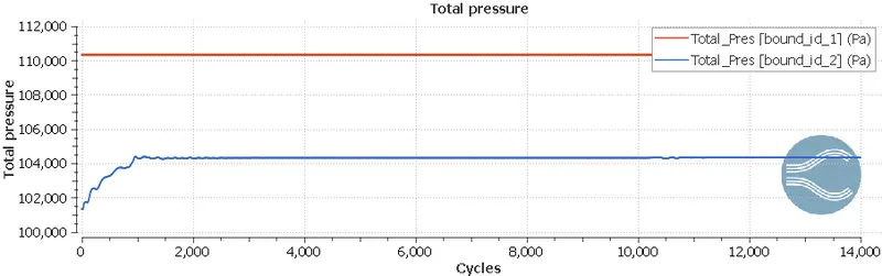 |
| Mass flow rate | 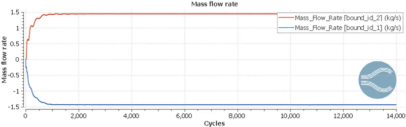 |
| Cell count | 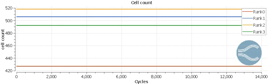 |
| Case 2 | |
| Velocity | 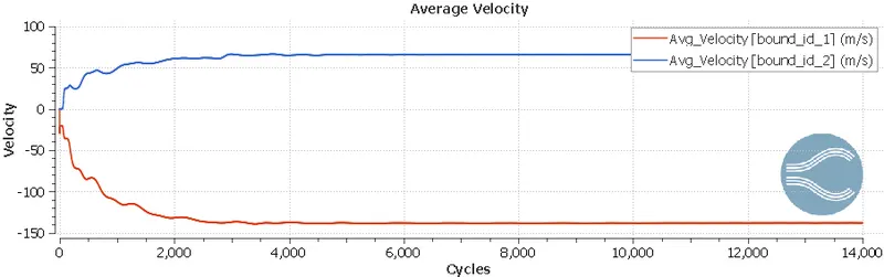 |
| Pressure | 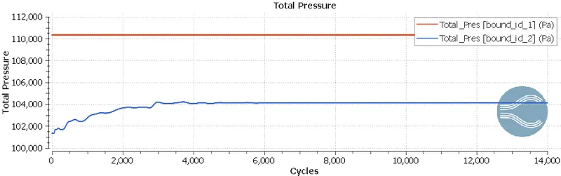 |
| Mass Flow Rate | 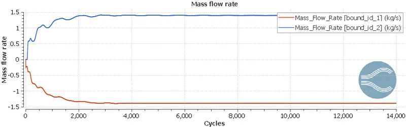 |
| Cell Count | 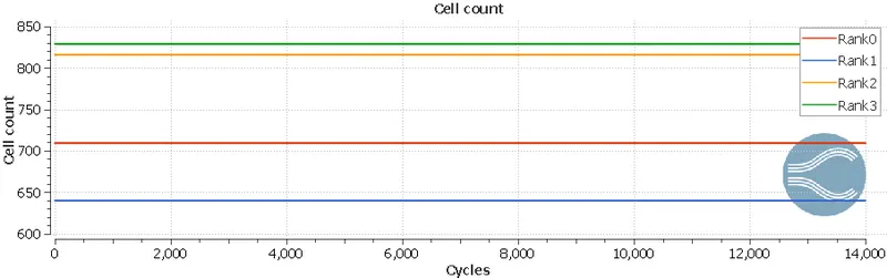 |
| Case 3 | |
| Velocity | 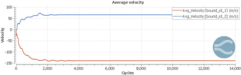 |
| Pressure | 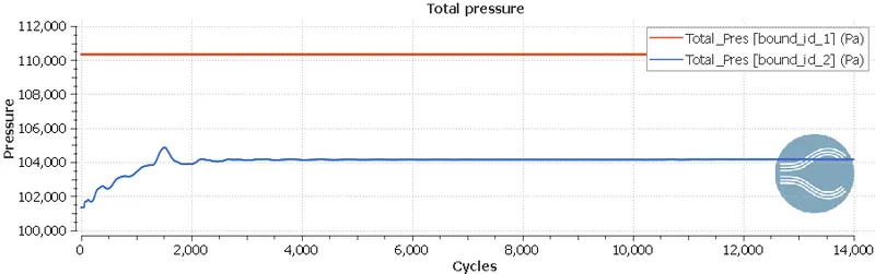 |
| Mass Flow Rate | 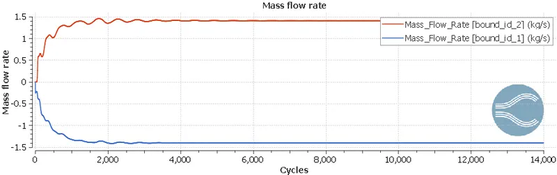 |
| Cell Count | 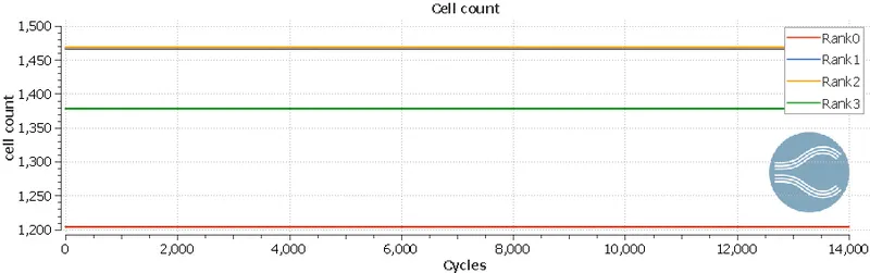 |
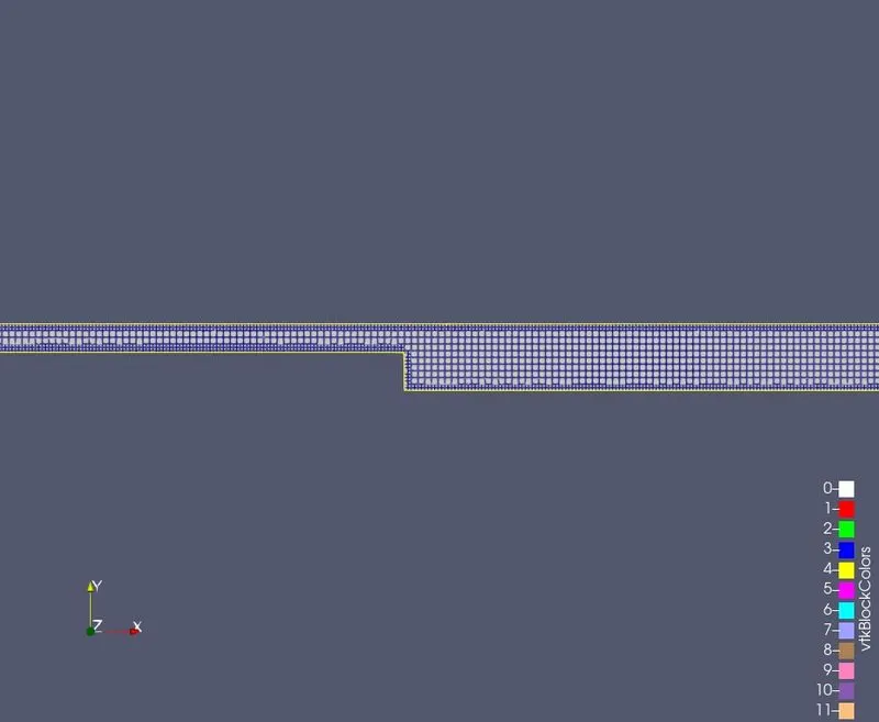
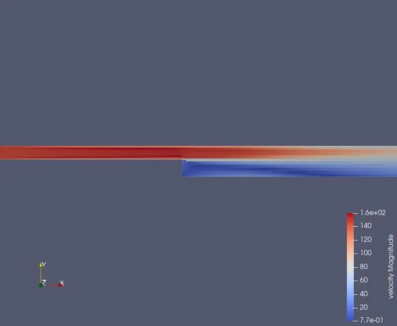
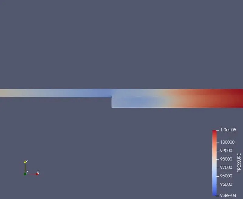
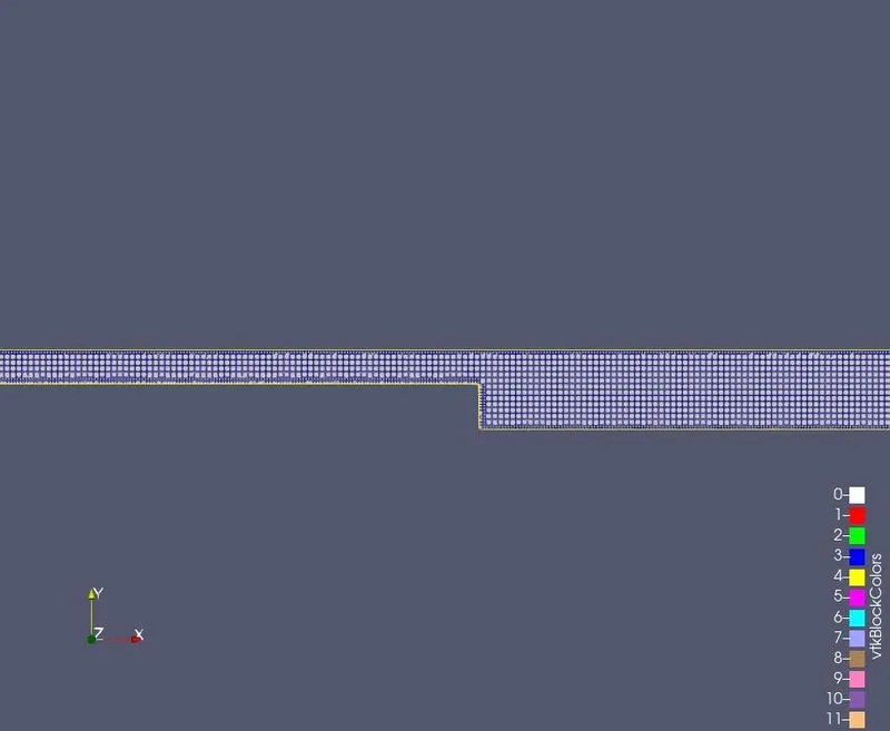
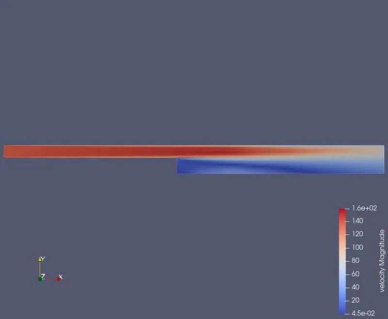
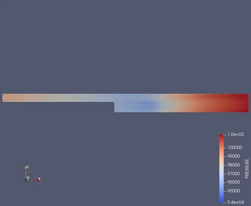
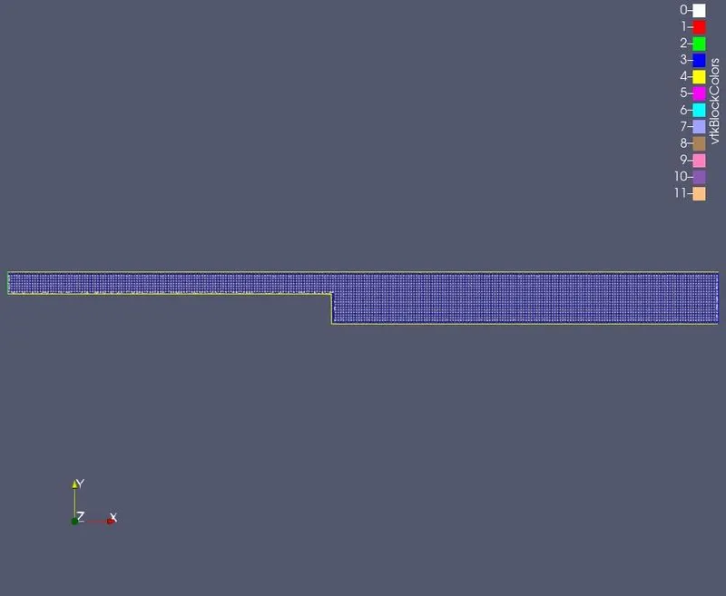
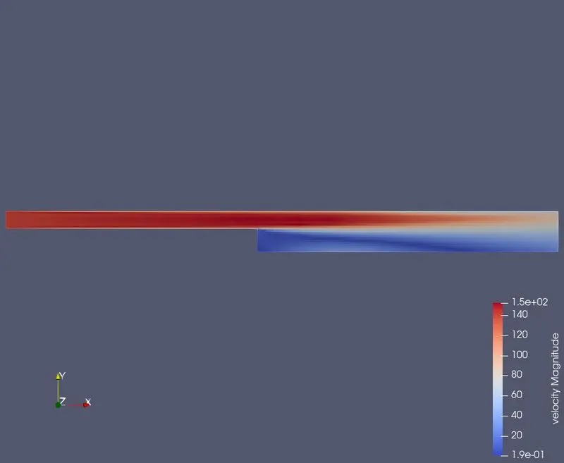
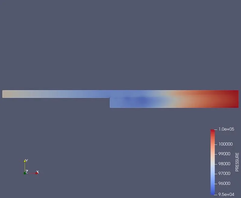
Contures of grid, velocity and pressure frm Paraview.
Case 1
|
|||
|
Case 2
|
|||
|
Case 3
|
Velocity and Pressure animation for each case.
|
Case 1 |
||
|
Case 2 |
||
|
Case 3 |
Flow separation: The phenomenon of flow separation occurs in situation when a pressure difference is generated or the shape of the body is not streamlined or there is abrupt edge on the body. This is detrimental to the aerodynamical performace of the body.
An adverse pressure is created which leads to reversal of the flow but due to the high speed on oncoming flow form upstream it does not flow back. Hence, flow separetes. Besides this increasing Reynold's number is also a factor leading to flow separation.
Due to the separation at the bottom of the step ther is lower velocity and also which developes high pressure (adverse pressure) which lead to flow separation.
The following probem shows the effect of backwards step on flow, from flow separetion to the mass flow rate and velocity of the flow. It can be seen that as the number of cells incease the cycles taken by the solvers to stabilize the simulation is less. i.e as the number of cells increase the iteration for the solution to converge is less.