Week 9 - FVM Literature Review

Content

Sr No	Topic
1	Finite Voume Method
1.1	Comparision
1.2	Steps to solve FVM
2	Interpolation
3	Flux Limiter

1) Finite Volume Method

Finite Volume Method is a Discretisation method that accounts for 3D arbitary shapes. Unlike FDM which is used to create an approximate algebric equation of well defined geometry, FVM makes it easy for the user to discrityze the equations using the control volume method(Itegrated form of the governing equations).

The arbitary shapes are broken down into mesh with well defined elements. These elements act as Control Volume(CV) and the equations are solved for these CVs. Then the results are integrsted over the geometry.

The equation that are solved inside the CVs are averaged for each element.

1.1) COMPARISION

As we take a look at FEM and FDM we can see both are discritization methods to solve a CFD problem. But we can compare them to understand the nuances of both methods.

Finite Difference Method	Finite Volume Method
Is good for a well defined geometry	Is good for an arbitary geometry as well
Grid is constructed to solve governing equations	Mesh comprising of elements id used ans the governing equations are integrated for all elements.
Discretisation is done for 1D and 2D	Discretisation can be done in 1D, 2D and 3D. Depending on the probelm.
Does not represent the governing equations properties accurately	Represents the governing equation properties more accurately(conservation, boundedness, transportativeness)

Above are some important points that cover the differences of both the methods.

To further illustrate FVM a 1D heat conduction equation will be used:

1D HEAT CONDUCTION EQUATION

`d/dx(Gammadphi/dx)+S = 0`

where,

`Gamma` : diffusion coefficient

S : Sourse term

`phi` : Function

1.2) Steps to solve FVM:

Steps involved in solving the equation

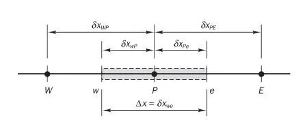
1) Grid generation: The geometry will be divided along its length at equal interval `trianglex`.

.

here the point W, P, E are the points at the center of the Control Volume. where w, e are the boundary of the control volume in contact with the boundary of P's CV. The distance between the 2 nodes is given by dx(WP), dx(PE) and dx(we).

2) Discretisation: This an important step to get closer to the simulation/ solution. The further steps help us assess the diffriential equation in a nwe light.

integrating the equation over the control volume. As we integrate over the range of(from west boundary of P to east boundary of P). The source term can be written in the `StriangleV`.

We obtain,

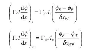
as we integrate we obtain the RHS terms using central difference method. Where the Diffusion terms are obtained by Linear Interpolation.

Here, the source term can be written as,

`StriangleV = Su + Sp phip`.

Finally the discrityzed equation looks like:

The general form of the equation can be written as:

3) Solution of the equation:

As the above equation is obtained for one node , same will be done for all other nodes and will be solved using iterative solvers.

For the points/nodes at the source appropriate boundary conditions will be applied.

2) INTERPOLATION

The Calculus that is representing the equation can't be interpreted by a computer, so we convert it into algebric form, This gives a pretty good estimate of original equation but there is also a large source of error. The size of the grid depends on the accuracy of equation.

The example of the source terms and the diffusion/ convection terms in our 1D equation as they are a function of temperature it is ncessay for them to be linearise.

Interpolation can help in briding the gap for calculus and simulation.

Depending on the order of interpolation can be first order, second order and higher order.

linear order interpolation is first order because it take 2 nearby points.

Another important aspect of interpolations is the nearby points. Closer the nearby points the better stablilty of the solution.

3) FLUX LIMITER

In a problem, there can be a senario where we have to bound the values of the terms(primitive variables). Eg in shock capturing the variables might jump to large values nad might cause unstability in the solution. To avoid this Flux limiters are used, they bound the values and not let them jump to a large values to cause any problem.

In engineering application it is necessay to have realistic values while simulation of abnormilities/Discontinuities. Flux limiters are algebric form to contain these problem.

here,

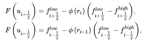
represents the edge flux if the ith cell. Where `phir`is the flux limiter function.

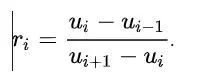
this is the successive gradient of solution mesh.