Solving the steady and unsteady 2D heat conduction problem.
Theory: In a problem involving change that takes plcae as time goes by it is necessary to see its effects as time passes. As the solution approaches to a state it won't change any further this is what we call a Steady state. Many a time it is important to understand the effects to time passing on a process. This process of analysing the process of simulating the process thorugh time is a Transient process.
As in this problem we will be analysing a second-order-PDE for 2D Heat conduction given by:
`(delT)/(delt) = c*((del^2T)/(delx^2)+(del^2T)/(dely^2))`
This equation represents the heat conduction through a 2D domain. As one can notice the presence of the "t" in the equation one can understand it is a time dependent process. This meanse this is a Transient process.
For Steady state as mentioned in the definition above the equation goes:
`(del^2T)/(delx^2)+(del^2T)/(dely^2)=0`
This means the equation is no longer dependent on the time.
Methodology:
As the Transient and Steady state analysis go there are ways to solve these problems, Why do we need these methods? as we will see the algebric forms of these equations annd further investigate the method of solving we will know the requirement of the number of methods to solve.
There are 2 major methods to solve the equations:
| Explicit | Implicit |
| 1) Jacobian | |
| 2) Gauss-Seidel | |
| 3) SOR |
Explicit and Implicit methods are used while time marching or Transient analysis. But for steady state we use Jacobian, Gauss-Seidel, SOR methods directly till convergence is reached.
Explicit method:
As in a time marching problem we calculate for a next timestep, to calculate this we can use the values from previous timesteps, this method we have only one unkown to solve for, these equation can be solved Explicitly.
for example of 1D heat conduction(for ease of understanding):

The term in RHS the what we calculate for next timestep(n+1) and we have known values of terms in LHS.
Implicit method:
An implict method involves only one known term and the rest are for the next timestep(unknown).

This is simple form of the equation where A,B,K are constants.
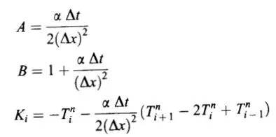
As we can observe the presence of 3 unknown terms in the equation it is immpossible to slove them.Unless we find the equation for other grid points so that we can create a system of coupled linear equation.
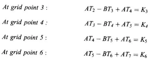
This methodcan be solved using matrix inversion method.
The matrix obtained will look like:
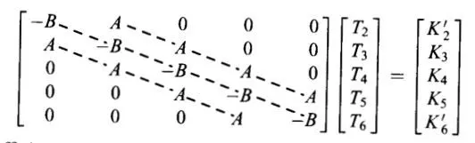
Although, there are 3 methods to solve the system of equation using
1) Jacobian method
2) Gauss-Seidel method
3) SOR (Successive over-Relaxation)
These 3 are iterative method which compare the calculated the error in a loop and compare it with a tolerence value.As the error falls below the tolerance we consider the convergence is achieved.
In a nutshell the iterative methods are given below:
- Jacobi method involves the computation of the of the current term using the values obtained in the previous term.
- The computation of x(k+1) uses the elements of x(k+1) that have already been computed, and only the elements of x(k) that have not been computed in the k+1 iteration. This means that, unlike the Jacobi method, only one storage vector is required as elements can be overwritten as they are computed, which can be advantageous for very large problems.
A relaxation factor is introduce provides a faster way to converge. For the current project we use 1.2 as the relaxation factor. `Tcurrent = (1-omega)*Told + omega*(Tgs)`(Tgs = Tgauss-seidel)
---------------Transcient method---------------
Code for Transient Analysis(Explicit method):
function time = c_trnsient_explicit(Solver)
    %Transient Explicit
    L = 1; %length of sides(equal as domain is square)
    nx = 10; %Nodes in x
    ny = 10; %Nodes in y
    c = 1.4; %Alpha
    dt = 1e-4; %timestep

    %Creating nodes indomain for x, y
    x = linspace(0, 1, nx);
    dx = L/(nx-1);

    y = linspace(0, 1, ny);
    dy = L/(ny-1);

    %Temperature profile
    T = 300*ones(nx, ny); %Initial Guess

    %boundary conditions for edges and corners
    %edges
    T(1, 2: end-1) = 600; %top
    T(end, 2:end-1) = 900; %bottom
    T(2:end-1, 1) = 400; %left
    T(2:end-1, end) = 800; %right
    %corners
    T(1, 1) = (600 + 400)/2; %Top left
    T(end, 1) = (900+400)/2; %Bottom left
    T(1, end) = (600+800)/2; %Top right
    T(end, end) = (900+800)/2; %Bottom right

    %copying the temperature.
    Told = T;

    %Defining variable for formula
    k1 = c*dt/(dx^2);
    k2 = c*dt/(dy^2);
    term_1 = 1/(1+2*k1+2*k2);
    term_2 = k1*term_1;
    term_3 = k2*term_1;


    if Solver == 1
        tic
        for t = 1:1400
            for i = 2:nx-1
                for j = 2:ny-1
                    %equation explicit.
                    T(i, j) = Told(i, j) + k1*(Told(i-1, j) - 2*Told(i,j) + Told(i+1, j)) + k2*(Told(i, j-1) - 2*Told(i,j) + Told(i, j+1));
                end
            end
            %Error's Maximum value
        error = max(max(abs(Told-T)));

        %Updating the temperature profile
        Told = T;


        end
        %Timing the loop to know the time requaited for whole steps.
        time = toc;
    end

%Plotting the solution at steady state.
    figure(1)
    [xx, yy] = meshgrid(x, y);
    [t, h] = contourf(xx, yy, T);
    set(gca,'Ydir', 'reverse')
    clabel(t, h);
    title({"Transient state explicit solver, time(s): ", num2str(time)})
end
%Solver = 1 To initiate the explicit method
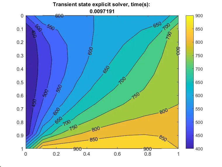
Output: Time taken by the Explicit solver to reach steady state.
Code for Transicent analysis(Implicit method):
function [iter, time] = c_transient_implicit(Solver)
%The function will return the number of iterations performes by every
% clear all
% close all
% clc
%
% Solver = 1;
%inputs
L = 1; %length of side(sme for x and y since it is a square)
nx = 10; %Number of nodes on X
ny = 10; %Number of nodes on Y
tol = 1e-4; %Tolerance for convergence
dt = 1e-4; %timestep
c = 1.4; %alpha

%Defining Domain and dx, dy.
x = linspace(0, 1, nx);
dx = L/(nx-1);
y = linspace(0, 1, ny);
dy = L/(ny-1);

%Defining the Temperature profile
T = 300*ones(nx, ny);

%Boundary conditions at edges and corners.
%Edges
T(1, 2: end-1) = 600; %top
T(end, 2:end-1) = 900; %bottom
T(2:end-1, 1) = 400; %left
T(2:end-1, end) = 800; %right
%Corners
T(1, 1) = (600 + 400)/2; %Top left
T(end, 1) = (900+400)/2; %Bottom left
T(1, end) = (600+800)/2; %Top right
T(end, end) = (900+800)/2; %Bottom right

%Making a copy of Temperature.
Told = T;
T_prev = T;

%Defining the formula interms of variables.
k1 = c*dt/(dx^2);
k2 = c*dt/(dy^2);
term_1 = 1/(1+2*k1+2*k2);
term_2 = k1*term_1;
term_3 = k2*term_1;
iter = 1; %initial iteration
t_1 =1; %simulation time
n = t_1/dt; %Total time steps

if Solver == 1 %Jacobi Method
    name = 'Jacobi';
    tic
    for nt = 1:n %Timestep for each step
        error = 1; %Initial error

        %Convergence loop compars the error with tolerance
        while error>tol
            %Solving for i, j
            for i = 2:nx-1
                for j = 2:ny-1
                    H = (Told(i-1, j)+Told(i+1, j));
                    V = (Told(i, j-1)+Told(i, j+1));
                    T(i,j) = T_prev(i,j)*term_1 + H*term_2+V*term_3; %Representing the formula
                end
            end
            %Calculating the error's maximum value
            error = max(max(abs(Told-T)));
            %Updating the values
            Told = T;
            %Iteration counter
            iter = iter +1;
        end
        T_prev=T;
    end
    time = toc;

end

if Solver == 2 %Gauss-Seidel Metlod
    name = 'Gauss-Seidel';
    tic
    for nt = 1:n %Time steps for each step
        error = 1;
        while error>tol
            for i = 2:nx-1
                for j = 2:ny-1
                    H = (T(i-1, j)+Told(i+1, j));
                    V = (T(i, j-1)+Told(i, j+1));
                    T(i,j) = T_prev(i,j)*term_1 + H*term_2+V*term_3;
                end
            end
        %Calculating the error's maximum value
        error = max(max(abs(Told-T)));
        %Updating the values
        Told = T;
        %Iteration counter
        iter = iter +1;
        end
        T_prev = T;
    end
    time = toc;

end

if Solver == 3 %SOR
    name = 'SOR';
    omega = 1.01; %Defining the Omega.
    tic
    for nt = 1:n %Timestep for each step
        error = 1;
        while error>tol
            for i = 2:nx-1
                for j = 2:ny-1
                    H = (T(i-1, j)+Told(i+1, j));
                    V = (T(i, j-1)+Told(i, j+1));
                    T(i, j) = (1-omega)*Told(i, j)+omega*(T_prev(i,j)*term_1 + H*term_2+V*term_3);
                end
            end
        %Calculation of maximum value of error
        error = max(max(abs(Told-T)));
        %Updating the value
        Told = T;
        %iteration counter
        iter = iter +1;
        end
        T_prev = T;
    end
    time = toc;
 end

%Plotting the Contour plot.
figure(1)
[xx, yy] = meshgrid(x, y);
[t, h] = contourf(xx, yy, T, ':');
set(gca,'Ydir', 'reverse')
clabel(t, h);
colorbar
xlabel("X-Axis")
ylabel("Y-Axis")
title({"Transient state implicit solver";['for: ', name]; ['time(s):', num2str(time)]; ['iterations: ' num2str(iter)]}) %num2str converts int to string
end
%Solver: 1 = Jacobi
%2 = Gauss_seidel
%3 = SOR
%To initiate the solver of choice
Output: Solution for steadiness
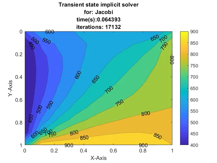
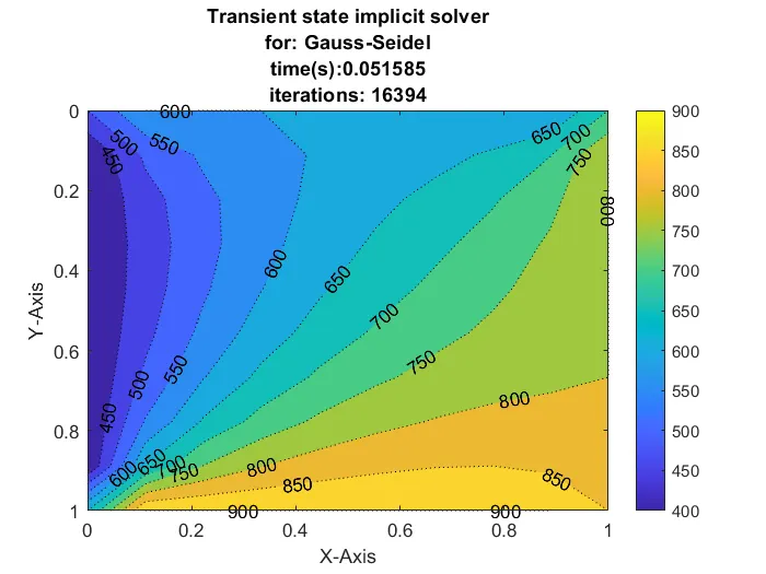
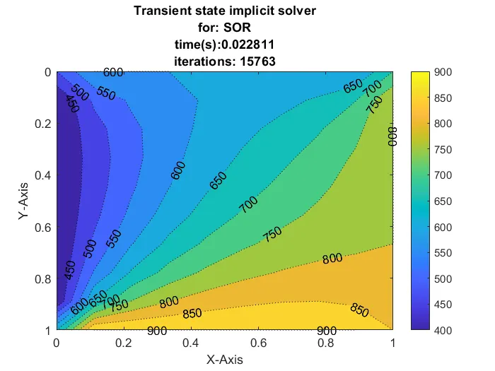
Jacobi > Gauss-Seidel>SOR
---------------Steady state method---------------
Steady state analysis:
function iter = c_steady_state_2D_heat_conduction(Solver)
%The function will return the number of iterations performes by every
%Solver.

%inputs
L = 1; %length of side(sme for x and y since it is a square)
nx = 50; %Number of nodes on X
ny = nx; %Number of nodes on Y
tol = 1e-4; %Tolerance for convergence

%Defining Domain and dx, dy.
x = linspace(0, 1, nx);
dx = L/(nx-1);
y = linspace(0, 1, ny);
dy = L/(ny-1);

%Defining the Temperature profile
T = 300*ones(nx, ny);

%Boundary conditions at edges and corners.
%Edges
T(1, 2: end-1) = 600; %top
T(end, 2:end-1) = 900; %bottom
T(2:end-1, 1) = 400; %left
T(2:end-1, end) = 800; %right
%Corners
T(1, 1) = (600 + 400)/2; %Top left
T(end, 1) = (900+400)/2; %Bottom left
T(1, end) = (600+800)/2; %Top right
T(end, end) = (900+800)/2; %Bottom right

%Making a copy of Temperature.
Told = T;

k = (2*(dx^2+dy^2))/(dx^2*dy^2); %Defining the formula interms of variables.

iter = 1;
if Solver == 1 %Jacobi Method
    name = 'Jacobi';
    error = 1;
    %Convergence loop compars the error with tolerance
    while error>tol
        %Solving for i, j
        for i = 2:nx-1
            for j = 2:ny-1
                H = (Told(i-1, j)+Told(i+1, j));
                V = (Told(i, j-1)+Told(i, j+1));
                T(i, j) = (1/k)*(H/dx^2)+(1/k)*(V/dy^2); %Representing the formula
            end
        end
        %Calculating the error's maximum value
        error = max(max(abs(Told-T)));
        %Updating the values
        Told = T;
        %Iteration counter
        iter = iter +1;
    end
end

if Solver == 2 %Gauss-Seidel Metlod
    name = 'Gauss-Seidel';
    error = 1;
    while error>tol
        for i = 2:nx-1
            for j = 2:ny-1
                H = (T(i-1, j)+Told(i+1, j));
                V = (T(i, j-1)+Told(i, j+1));
                T(i, j) = (1/k)*(H/dx^2)+(1/k)*(V/dy^2);
            end
        end
        %Calculating the error's maximum value
        error = max(max(abs(Told-T)));
        %Updating the values
        Told = T;
        %Iteration counter
        iter = iter +1;
    end
end

if Solver == 3 %SOR
    name = 'SOR';
    omega = 1.2; %Defining the Omega.
    error =1;
    while error>tol
        for i = 2:nx-1
            for j = 2:ny-1
                H = (T(i-1, j)+Told(i+1, j));
                V = (T(i, j-1)+Told(i, j+1));
                T(i, j) = (1-omega)*Told(i, j)+omega*((1/k)*(H/dx^2)+(1/k)*(V/dy^2));
            end
        end
        %Calculation of maximum value of error
        error = max(max(abs(Told-T)));
        %Updating the value
        Told = T;
        %iteration counter
        iter = iter +1;
    end

end

%Plotting the Contour plot.
figure(1)
[xx, yy] = meshgrid(x, y);
[t, h] = contourf(xx, yy, T, ':');
set(gca,'Ydir', 'reverse')
clabel(t, h);
colorbar
xlabel("X-Axis")
ylabel("Y-Axis")
title({"Steady state solver";['for: ', name]; ['iterations: ' num2str(iter)]}) %num2str converts int to string

end
%Solver: 1 = Jacobi
%2 = Gauss_seidel
%3 = SOR
%To initiate the solver of choice
Output:Solution for steadiness
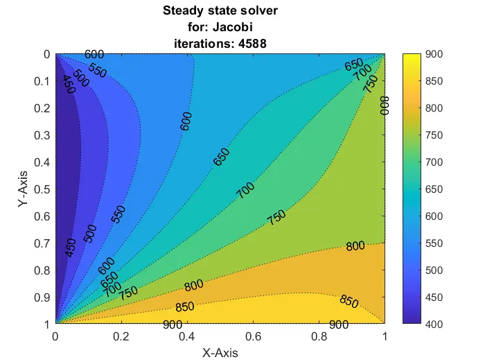
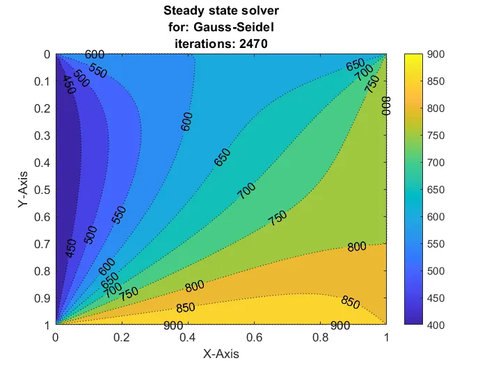
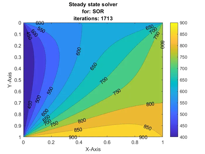
Jacobi > Gauss-Seidel>SOR
-------------------------------------End of code and outputs-------------------------------------
Comments on the output:
As it is evident with the outputs and comparing the iterative methods we can clearly see that the iterations have an order. Jacobi>Gauss-Seidel>Successive over-relaxation.
Furthermore from the outputs for transient analysis we can also see the time requaired for explicit and implicit method. Although the variation of the inputs will affect the solution, the fact that these solution reach a steady state is inevitable. As for the unstability goes by varying the time steps(explicit, implicit) and varying the dx, dt(steady state) the solution can become unstable. This depends on the CFL number of the equation as well.
As an example the plot below shows the unstability condition:
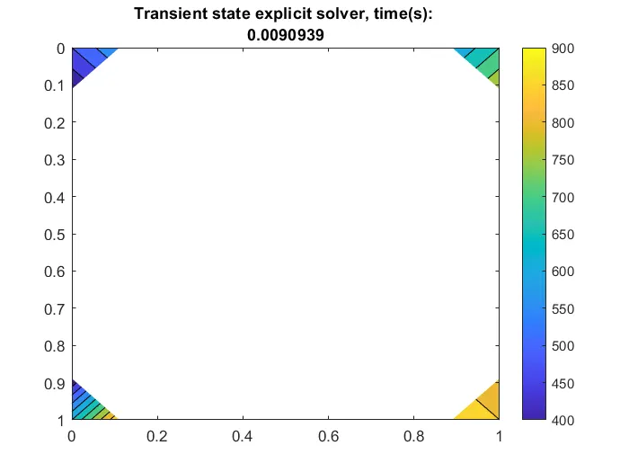
Above is a Transient analysis explicit method with time step taken as 1e-4. This increases the value of the Courant number(CFL) by the requaired for the equation and hence we get an unstable/unrelaiable solution.
Conclusion:
Here we solved a 2D heat conduction equation by using various iterative methods, implicitly and explicitly. We also understood the transient and steady state approach and touched upon the iterative methods.