Week 1- Mixing Tee

Content Sr No Topic 1 Introduction 2 Mesh Configuration 3 Short T Mesh 3.1.a K-Epsilon vs K-Omega (Mr: 2) 3.1.b Reason to choose solver 3.2 Short T Momentum Ratio: 4 4 Long T Mesh 4.1 Momentum Ratio: 2 4.2 Momentum Ratio: 4 5 Mesh Independence test 6 Comment on the result (Length and Momentum Ratio) 7 Conclusion

------------------------------------------------------------------

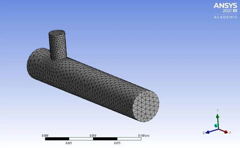
1) Introduction: Ansys fluent is a close source software to solve CFD problems. In this report an attempt is made to simulate a Mixing T of 2 geometires(Short and Long) and dunderstand the accuracy of the simulation using the post processing tool in the software.

The steps followed are as follows:

Step 1	Geometry defining
Step 2	Meshing
Step 3	Setup(Solver, Boundary conditiions, Initial conditions)
Step 4	Post processing

------------------------------------------------------------------

2) Mesh Configuration

	Short T	Long T
Element size	0.005	0.005
Number of elements	14247	17787

------------------------------------------------------------------

3) Mesh for short T

------------------------------------------------------------------

3.1) Short T Momentum ratio: 2

3.1.a) K-Epsilon vs K-Omega

Sr No	K-Epsilon	K-Omega
Residual
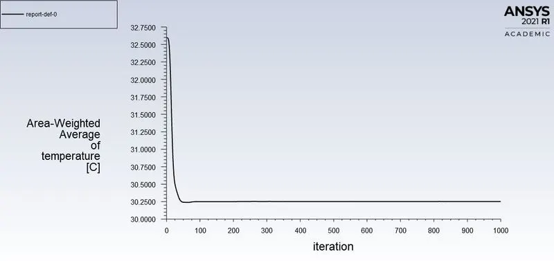
Area Weighted average of temperature
Standard Deviation of Temperature at outlet

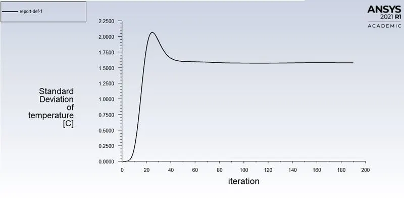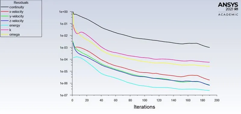
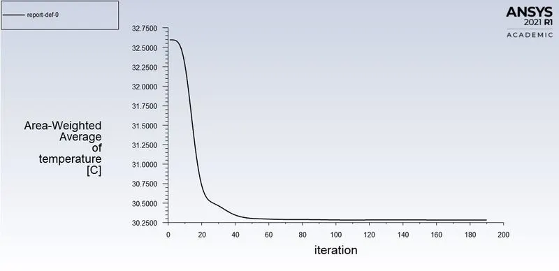
Solution converged for K-Omega:

------------------------------------------------------------------

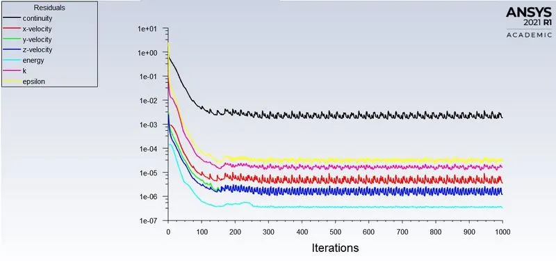
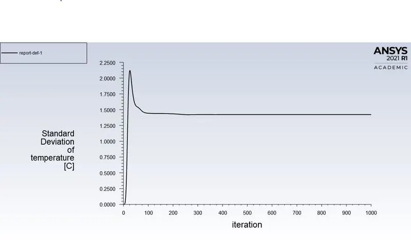
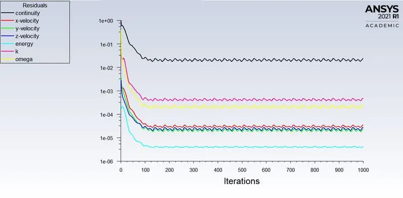
3.1.b) Reason to select K-Omega: As from above result it can be observed that the solution converged for K-Omega, also the residual for K-Epsilon are showing fluctuations and carried out till the 1000th iteration. Although, it can be said to have been converged but the fact that K-Omega actually converged without fluctuations gave the confidence of moving ahead with it. Also, the difference in Standard Deviation is small so it was not given as much importance to the seleection criteria.

------------------------------------------------------------------

3.2) Short T Momentum ratio: 4

Sr No	Image of plot
Residual
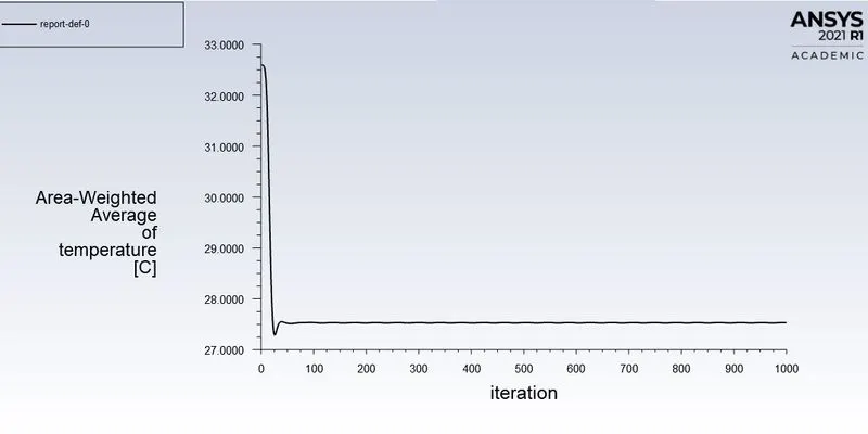
Area Weighted average of outlet temperature
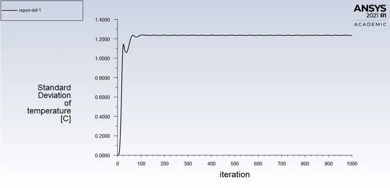
Standard deviation of outlet temperature

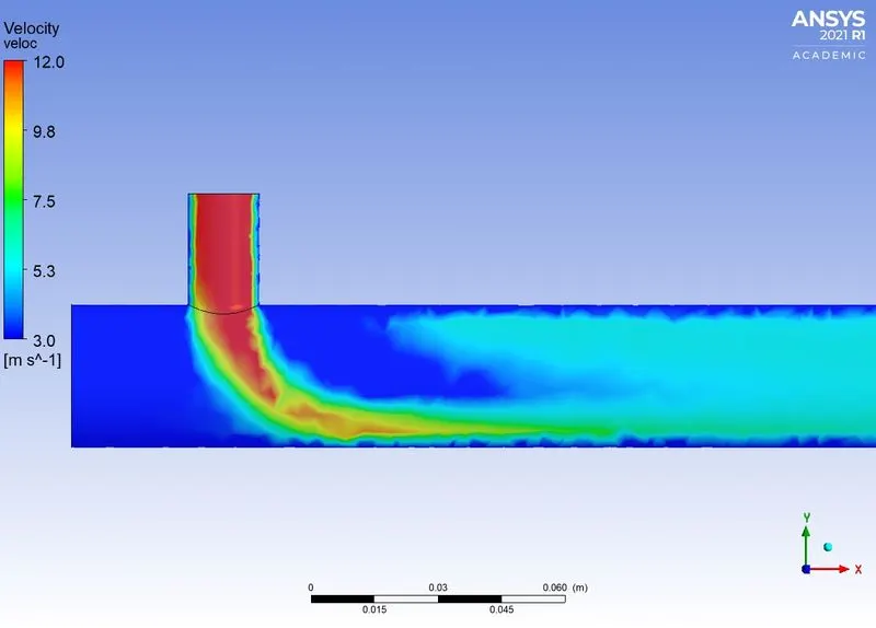
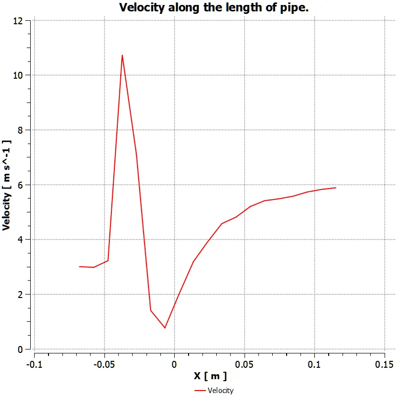
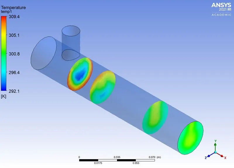
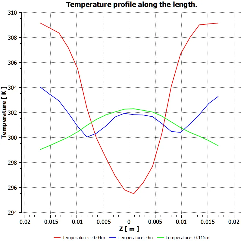
Post Processing

Sr No	Image	Plot
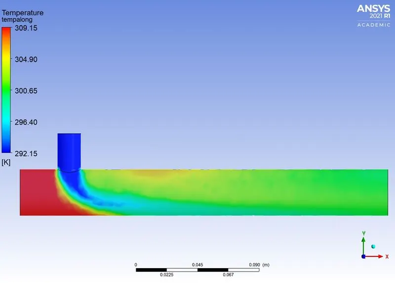
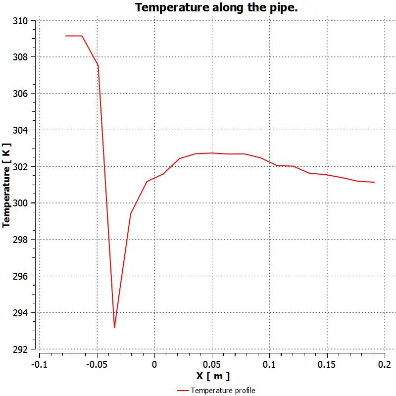
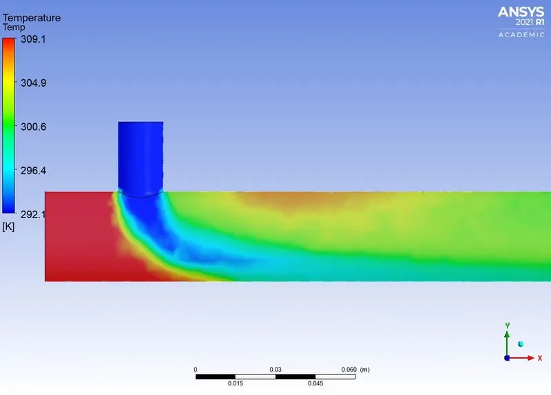
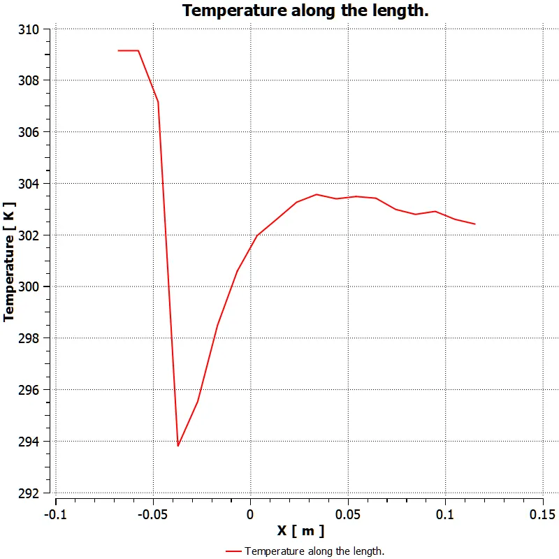
Temperature Along the length of pipe
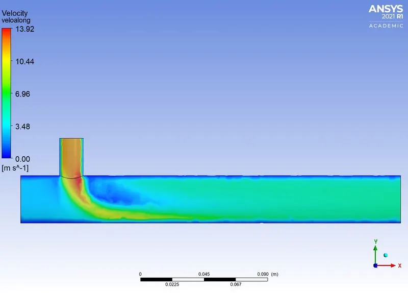
Velocity along the length of pipe
Temperature accross the pipe
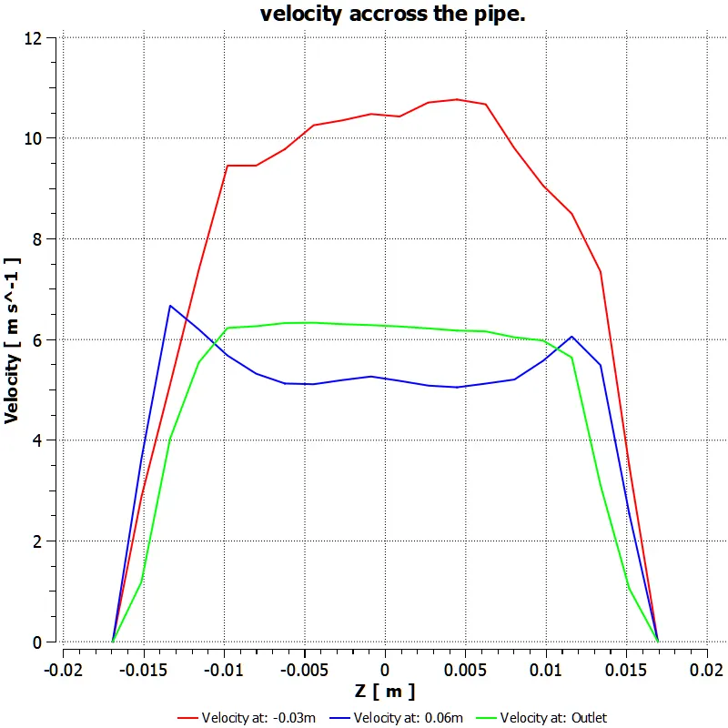
Velocity accross the pipe

------------------------------------------------------------------

4) Mesh for Long T

------------------------------------------------------------------

4.1) Long T Momentum ratio: 2

Sr No	Image of plot
Residual
Area Weighted average of outlet temperature
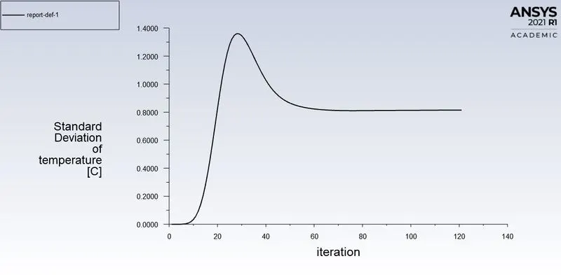
Standard deviation of outlet temperature

Iterations to converge

Post Processing

Sr No	Image	Plot
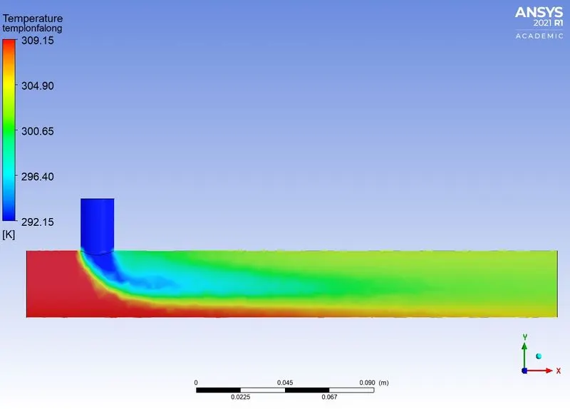
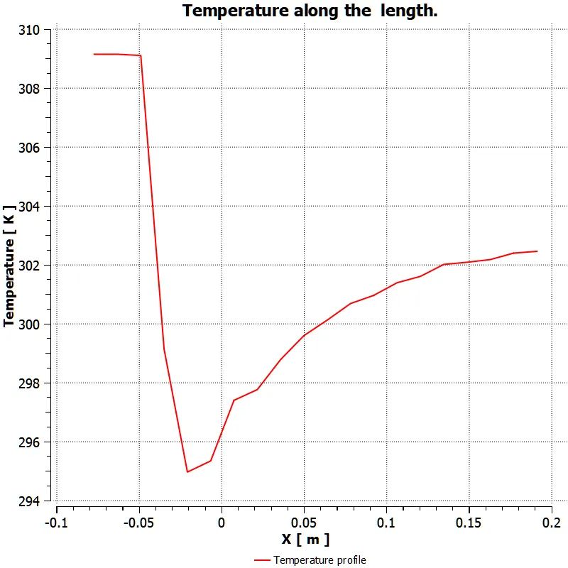
Temperature Along the length of pipe
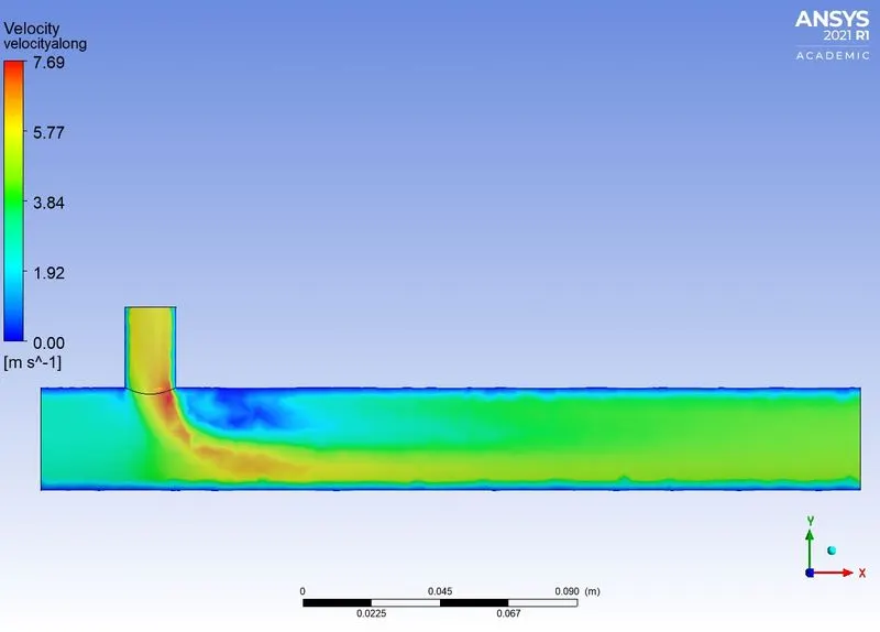
Velocity along the length of pipe
Temperature accross the pipe
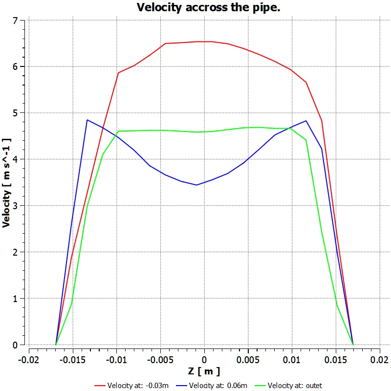
Velocity accross the pipe

------------------------------------------------------------------

4.2) Long T Momentum ratio: 4

Sr No	Image of plot
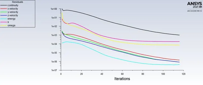
Residual
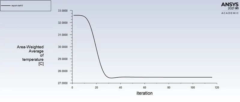
Area Weighted average of outlet temperature
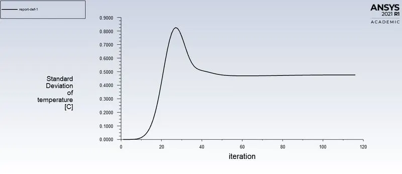
Standard deviation of outlet temperature

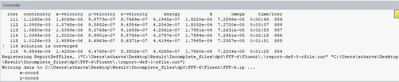
Iterations for convergence

Post Processing

Sr No	Image	Plot
Temperature Along the length of pipe
Velocity along the length of pipe
Temperature accross the pipe
Velocity accross the pipe

------------------------------------------------------------------

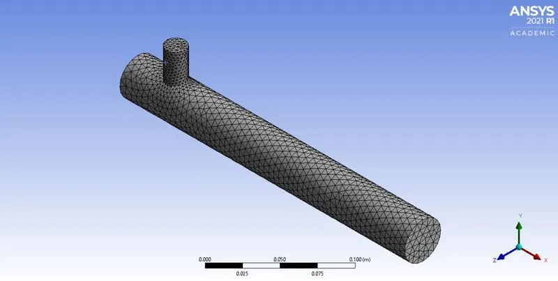
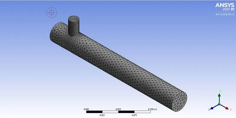
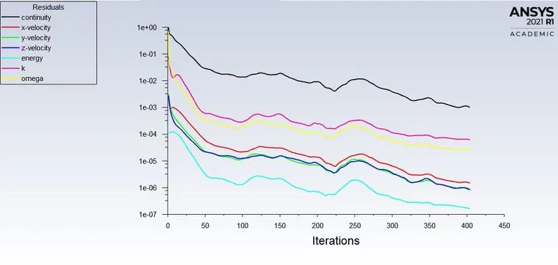
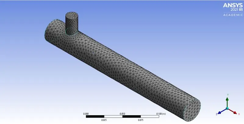
5) Mesh Independence test:

The configuratuon selected for this was long T:

The detailes of the simulation sat same as above (K-Omega). Also the boundary conditions and initial conditions are same as Long T for Momentum ratio: 2.

Mesh Configuration	Mesh	Residual
Default (1.39e-2)
0.008
0.005

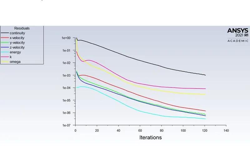
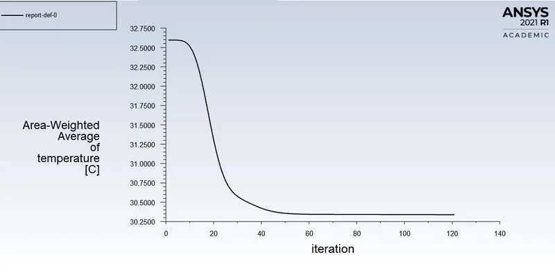
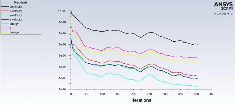
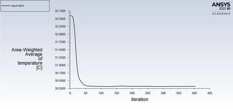
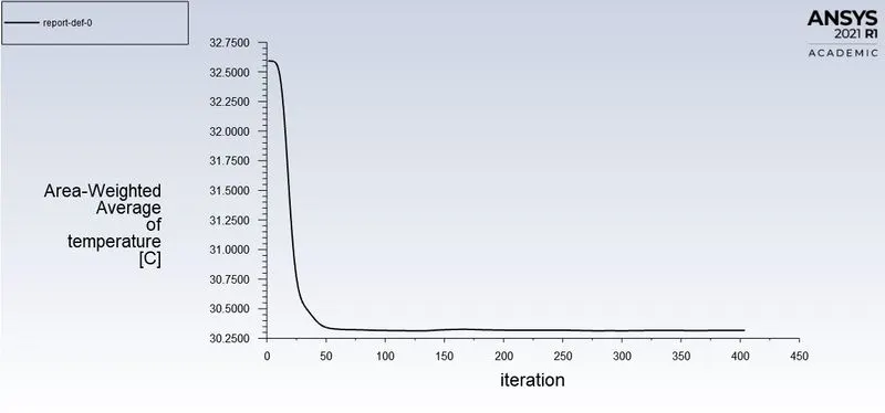
From above result we can observe the solution converges (initialted for 1000 iterations) at:

Mesh config	Iterations requaired to converge.	Average temperature
Default	404
0.008	400
0.005	121

As the solution converges it almost converges to the same value. Although it could be conclude that the mesh size does not affect the solution of average weighted temperature. This could mean the Mesh is independent of the solution. As in the case above, but it is worth noting that more refinement might change the final result and would also require lesser interations.

------------------------------------------------------------------

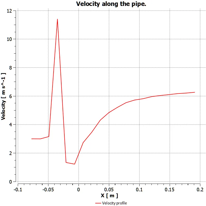
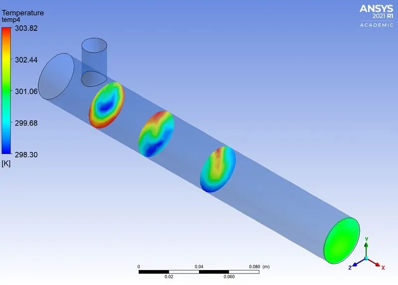
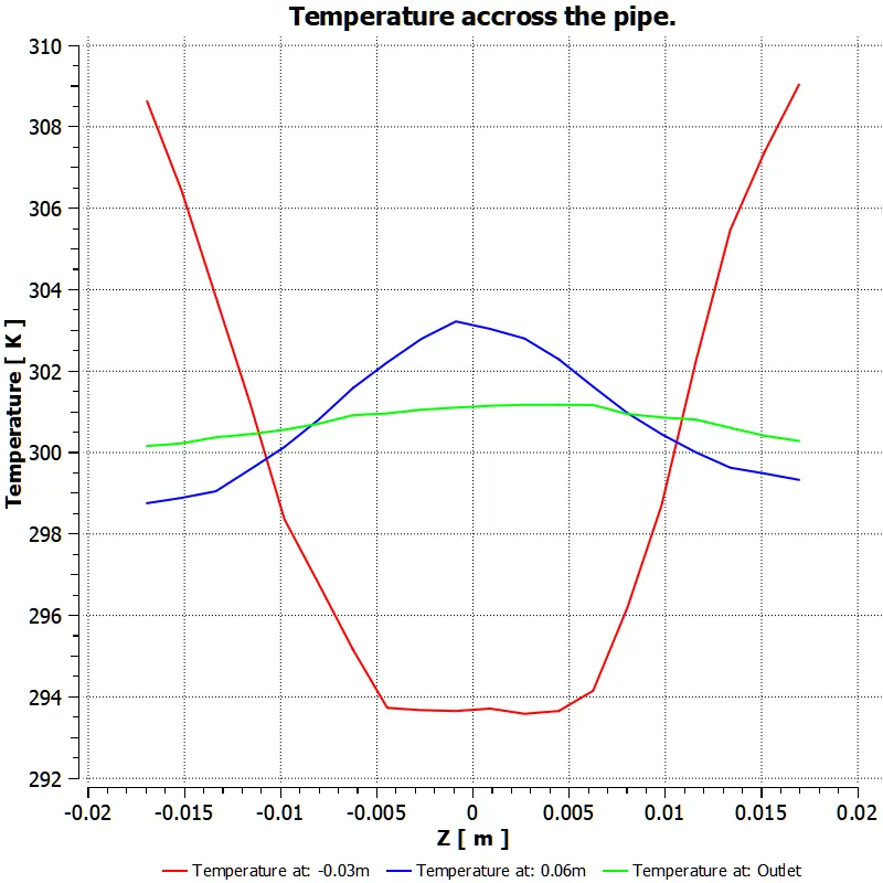
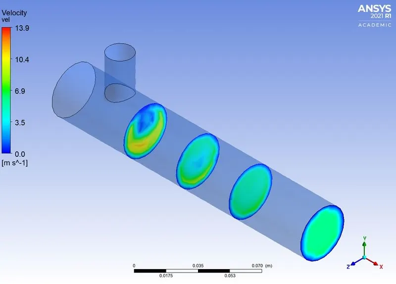
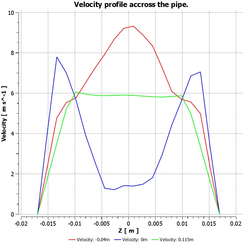
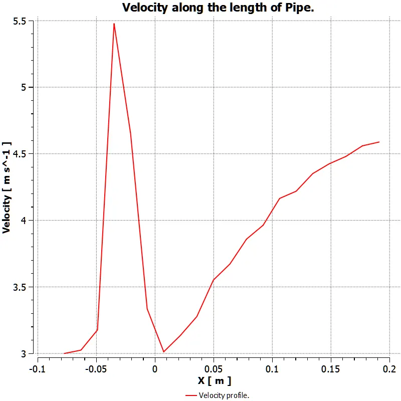
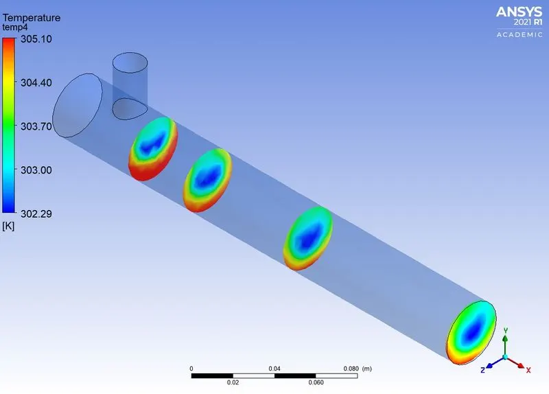
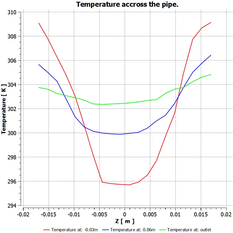
6) Comment on the results: As from all above the results it can be observed that in each cse there is slight difference that make the solution change slightly. Itis obvious that the mixing will be better as the length of the pipe is increased due to dissipation that occurs because of turbulance, more accurately as the wall is having substantial cause of turbulance (due to shearing stress/effect) the mixing occurs and heb=nce the temperature is more uniform in the long pipe. As for the short pipe is concerned the mixing is not as efficient due to shorter length.

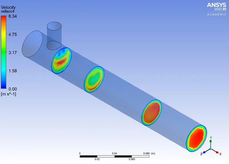
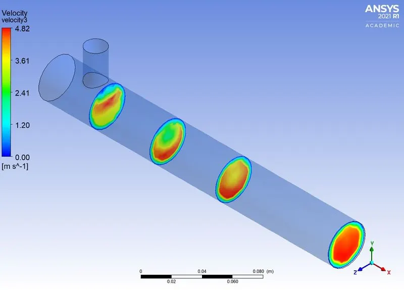
Plus, due to the high velocity in the second case (Momentum Ratio=4) the colder air flow is more dominant and the mixing does not occur as efficiently as well. Maybe that is why the the fluctuations occure for K-Omega in shorter pipe for Momentum ratio=4.

Note: For some solutions the contour plots might suggest a profile that seems more diffused or otherwise. It is beacuse of the settings changing in Ansys Fluent from Global/Local/User defined.

7) Conclusion: As above report shows the result and the render of the Mixing T for both geometry, it is concluded that the simualtion are successful.