|
Content
| Sr No. |
Topic |
| 1 |
Introduction |
| |
Analytical Solution |
| 2 |
Assumed values |
| 3 |
Steps to solve for Analytical Solution |
| 4 |
Analytical Solution |
| |
Simulation |
| 5 |
Automation |
| 5.1 |
Code for creating co-ordinate |
| 5.2 |
Code for creating blockMeshDict |
| 6 |
Simulation Files |
| 6.1 |
blockMeshDict |
| 6.2 |
pressure |
| 6.3 |
Velocity |
| 6.4 |
transportProperties |
| 6.5 |
controlDict |
| 7 |
preview and Simulation results |
| 8 |
Result and validation |
| 9 |
Comments on Result |
| 10 |
Conclusion |
|
Analytical Solution
1) Introduction: Understanding flow through pipe and comparing the analytical results with Simulations and validating them using OpenFoam.
For this we employ the help of Hagen-Poiseuille's Equation and Reynold number formula to evaluate the analytical solution.
2) Given and assumed values:
| Sr No. |
Properties |
Values |
| 1 |
Diameter of pipe(assumed) |
20mm |
| 2 |
Kinematic Viscosity |
`0.8926*10^-6 N*sm^-2` |
| 3 |
Density of water |
1000 `Kg/m^3` |
| 4 |
Reynolds Number |
2100 |
3) For our current probelm we make an assumption and use the diameter as an assumed value. The methodology of the problem is given below.
Step 1) Identify the entry length of the pipe.
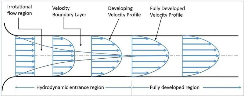
The hydrodynamic entrence length is given by: `0.05*Re*D` for Laminar flow.
using this we obtain the entry length. `Le`.
The length of the whole pipe is greater than Entry length. I.e Le < L.
Step 2) The velocity that is obtained analytically can be expressed using the Reynold's number, which is given by.
`Re = (v*D)/nu`
Reynolds number for Lan=minar flow is 2100 for water.
Step 3) Use the length of pipe to find the pressure difference accross the pipe.
Using Hagen–Poiseuille equation to find the Pressure Difference:`(32*L*nu*v)/D^2` using the Length obtained from above method we find the pressure difference accross the pipe.
The kinamatic pressure difference is given by: `(trianglep)/rho`
`rho = 1000` Density of water.
Step 4) Finding the shear across the wedge profile. Shear gives an idea of how the flow is occuring accross the cross-section of the pipe. The shear gives the profile of flow of the fluis through the pipe.
The equation is given by: `tau = (2*mu*v(max))/r`
4) Solution of Analytical solution.
Using all these steps we can obtain the values for analytical solution of flow through a pipe.
| Sr no No. |
Properties |
Values |
| 1 |
Le |
2.1m |
| 2 |
L |
2.5m |
| 3 |
Velocity(average) |
0.0935 m/s |
| 4 |
Velocity (maximum) |
0.1870m/s |
| 5 |
Pressure Drop |
16.6430 Pa |
| 6 |
Kinematioc Pressure Drop |
0.0166 Pa |
| 7 |
Shear Stress |
0.033 Pa |
The above process show the analytical method to evaluate the flow throught a pipe.
As far as the simulation and validation is concerned, it is Given below:
| ------------------------------------------------------------------ |
Simulation
The simulation method involves the use of OpenFoam and using MATLAB to automate the blockMeshDict file.
Using the values obtained from above like Diameter, Length of the pipe and the angle of the wedge.
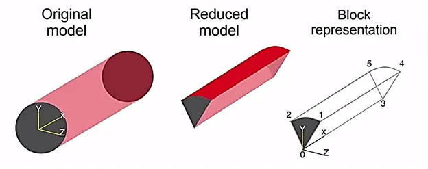
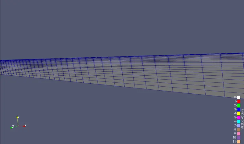
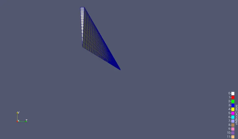
Angle of the wedge: As the simulation is axisymmetric it will be easier if we take as wedge instead of the whole pipe to make the simulation.
as the wedge is what will be used for simulation it is necessay to provide appropriate values to create a blockMesh file. For that the below code will automate the process.
5) Automation:
| 1) Code that calculates the co-ordinate points. |
function [points_t, points_b, x_arc, y_arc, zl] = new_bmd(ang, l, r);
%a function that reurns the co-ordinate points and co-ordinate of arc.

    %inputs

    zo = 0;
    zl = l;
    %creating the arrays for x, y co-ordinates
    x = linspace(0, r, 10);
    y = linspace(0, r, 10);

    %origin points
    xo = x(1);
    yo = y(1);

    %The points at the edge of wedge.
    xr = r*sind(ang);
    yr = r*cosd(ang);

    %Finding the points of the arc.
    ang_1 = linspace(0, ang, ang);
    for i = 1:length(ang_1)
        if ang_1(i) == 0
            x_arc = r*sind(ang_1(i));
            y_arc = r*cosd(ang_1(i));
        end
    end

    x_arc = x_arc;
    y_arc = y_arc;

    xl = -xr;
    yl = yr;

    %array that compiles the x, y, z co-ordinates
    a = [xo, yo, zo, xr, yr, zo, xl, yl, zo];
    b = [xo, yo, zl, xr, yr, zl, xl, yl, zl];


    arc = zeros(3, 3);
    arc_f = zeros(3,3);

    %Converting the points into an array and the length of the wedge is
    %along x-axis.
    for p = 1:length(a)
        arc(p) = a(p);
    end
    points_t = zeros(3, 3);
    points_t(1, :) = arc(3, :);
    points_t(2, :) = arc(2, :);
    points_t(3, :) = arc(1, :);

    for q = 1:length(b)
        arc_f(q) = b(q);
    end
    points_b = zeros(3, 3);

    points_b(1, :) = arc_f(3, :);
    points_b(2, :) = arc_f(2, :);
    points_b(3, :) = arc_f(1, :);
end
|
| 2) The code that creates a blockMeshDict file |
piy = fopen('C:UsersatharvaDesktop/blockMeshDict.txt', 'wt');
[points_t, points_b, x_arc, y_arc, zl] = new_bmd(3, 2.5, 0.01);

h = ["/*--------------------------------*- C++ -*----------------------------------*";
  "  =========                 |";
  "  \      /  F ield         | OpenFOAM: The Open Source CFD Toolbox";
  "   \    /   O peration     | Website:  https://openfoam.org";
  "    \  /    A nd           | Version:  8";
  "     \/     M anipulation  |";
"*---------------------------------------------------------------------------*/";
"FoamFile";
"{";
"    version     2.0;";
"    format      ascii;";
"    class       dictionary;";
"    object      blockMeshDict;";
"}";
"// * * * * * * * * * * * * * * * * * * * * * * * * * * * * * * * * * * * * * //";

"convertToMeters 1;";

"vertices"];


for i = 1:length(h)
    fprintf(piy, '%sn', h(i));
end
fprintf(piy, '(n');


for j = 1:3
    fprintf(piy, 't(%d %d %d)n', points_t(1:3, j)');
end
fprintf(piy, 'n');
for k = 1:3
    fprintf(piy, 't(%d %d %d)n', points_b(1:3, k)');
end
fprintf(piy, ');nn');
fprintf(piy, 'blocksn(n');
fprintf(piy, 'thex (%d %d %d %d %d %d %d %d) (500 20 1) simpleGrading (1 0.1 1)n);n', [0 3 5 2 0 3 4 1]);
fprintf(piy, 'edgesn(ntarc 1 2 (%d %d %d)ntarc 4 5 (%d %d %d)n);nn', [x_arc y_arc 0 zl y_arc 0]);
fprintf(piy, 'boundaryn(ntinletnt{ntttype patch;nttfacesntt(nttt(%d %d %d %d)ntt);nt}n', [0 1 2 0]);
fprintf(piy, 'toutletnt{ntttype patch;nttfacesntt(nttt(%d %d %d %d)ntt);nt}n', [3 5 4 3]);
fprintf(piy, 'ttopnt{ntttype wall;nttfacesntt(nttt(%d %d %d %d)ntt);nt}n', [1 4 5 2]);
fprintf(piy, 'tfrontnt{ntttype wedge;nttfacesntt(nttt(%d %d %d %d)ntt);nt}n', [0 3 4 1]);
fprintf(piy, 'tbacknt{ntttype wedge;nttfacesntt(nttt(%d %d %d %d)ntt);nt}n', [0 2 5 3]);
fprintf(piy, 'taxisnt{ntttype empty;nttfacesntt(nttt(%d %d %d %d)ntt);nt}n);n', [0 3 3 0]);
fprintf(piy, 'mergePatchPairsn(n);n');
fprintf(piy, '%s', "// ************************************************************************* //");
|
6) Setting up simulation in OpenFoam:
Using the blockMesh file obtained from automation will get the geometry, but there are various other tweaks need to be made to other files for better flow simulation.
The Files that are updated are:
| 6.1)blockMeshDict |
/*--------------------------------*- C++ -*----------------------------------*
  =========                 |
  \      /  F ield         | OpenFOAM: The Open Source CFD Toolbox
   \    /   O peration     | Website:  https://openfoam.org
    \  /    A nd           | Version:  8
     \/     M anipulation  |
*---------------------------------------------------------------------------*/
FoamFile
{
    version     2.0;
    format      ascii;
    class       dictionary;
    object      blockMeshDict;
}
// * * * * * * * * * * * * * * * * * * * * * * * * * * * * * * * * * * * * * //
convertToMeters 1;
vertices
(
	(0 0 0)
	(0 9.986295e-03 5.233596e-04)
	(0 9.986295e-03 -5.233596e-04)

	(2.500000e+00 0 0)
	(2.500000e+00 9.986295e-03 5.233596e-04)
	(2.500000e+00 9.986295e-03 -5.233596e-04)
);

blocks
(
	hex (0 3 5 2 0 3 4 1) (500 20 1) simpleGrading (1 0.1 1)
);
edges
(
	arc 1 2 (0 1.000000e-02 0)
	arc 4 5 (2.500000e+00 1.000000e-02 0)
);

boundary
(
	inlet
	{
		type patch;
		faces
		(
			(0 1 2 0)
		);
	}
	outlet
	{
		type patch;
		faces
		(
			(3 5 4 3)
		);
	}
	top
	{
		type wall;
		faces
		(
			(1 4 5 2)
		);
	}
	front
	{
		type wedge;
		faces
		(
			(0 3 4 1)
		);
	}
	back
	{
		type wedge;
		faces
		(
			(0 2 5 3)
		);
	}
	axis
	{
		type empty;
		faces
		(
			(0 3 3 0)
		);
	}
);
mergePatchPairs
(
);
// ************************************************************************* //
|
Done using automation |
| 6.2)pressure |
/*--------------------------------*- C++ -*----------------------------------*
  =========                 |
  \      /  F ield         | OpenFOAM: The Open Source CFD Toolbox
   \    /   O peration     | Website:  https://openfoam.org
    \  /    A nd           | Version:  8
     \/     M anipulation  |
*---------------------------------------------------------------------------*/
FoamFile
{
    version     2.0;
    format      ascii;
    class       volScalarField;
    object      p;
}
// * * * * * * * * * * * * * * * * * * * * * * * * * * * * * * * * * * * * * //

dimensions      [0 2 -2 0 0 0 0];

internalField   uniform 0;

boundaryField
{
    inlet
    {
        type            zeroGradient;
    }

    outlet
    {
        type            fixedValue;
        value	         uniform 0.0166;
    }

    top
    {
        type            zeroGradient;
    }

    front
    {
        type            wedge;
    }
    back
    {
        type            wedge;
    }
    axis
    {
        type            empty;
    }
}

// ************************************************************************* //
|
- Changing outlet pressure as obtained feom Hagen-Poiseuille's equation
|
| 6.3)Velocity |
/*--------------------------------*- C++ -*----------------------------------*
  =========                 |
  \      /  F ield         | OpenFOAM: The Open Source CFD Toolbox
   \    /   O peration     | Website:  https://openfoam.org
    \  /    A nd           | Version:  8
     \/     M anipulation  |
*---------------------------------------------------------------------------*/
FoamFile
{
    version     2.0;
    format      ascii;
    class       volVectorField;
    object      U;
}
// * * * * * * * * * * * * * * * * * * * * * * * * * * * * * * * * * * * * * //

dimensions      [0 1 -1 0 0 0 0];

internalField   uniform (0.0935 0 0);

boundaryField
{
    inlet
    {
        type            fixedValue;
        value	         uniform (0.0935 0 0);
    }

    outlet
    {
        type            zeroGradient;

    }

    top
    {
        type            fixedValue;
        value		 uniform (0 0 0);

    }

    axis
    {
        type            empty;
    }

    front
    {
        type            wedge;
    }
    back
    {
        type            wedge;
    }
}

// ************************************************************************* //
|
Substituting the obtained value of velocity in
- Internal field
- Inlet of the pipe
|
| 6.4)Transport properties |
/*--------------------------------*- C++ -*----------------------------------*
  =========                 |
  \      /  F ield         | OpenFOAM: The Open Source CFD Toolbox
   \    /   O peration     | Website:  https://openfoam.org
    \  /    A nd           | Version:  8
     \/     M anipulation  |
*---------------------------------------------------------------------------*/
FoamFile
{
    version     2.0;
    format      ascii;
    class       dictionary;
    location    "constant";
    object      transportProperties;
}
// * * * * * * * * * * * * * * * * * * * * * * * * * * * * * * * * * * * * * //

nu              [0 2 -1 0 0 0 0] 0.8926e-6;


// ************************************************************************* //
|
Defining the property of fluid i.e water |
| 6.5)ControlDict |
/*--------------------------------*- C++ -*----------------------------------*
  =========                 |
  \      /  F ield         | OpenFOAM: The Open Source CFD Toolbox
   \    /   O peration     | Website:  https://openfoam.org
    \  /    A nd           | Version:  8
     \/     M anipulation  |
*---------------------------------------------------------------------------*/
FoamFile
{
    version     2.0;
    format      ascii;
    class       dictionary;
    location    "system";
    object      controlDict;
}
// * * * * * * * * * * * * * * * * * * * * * * * * * * * * * * * * * * * * * //

application     icoFoam;

startFrom       startTime;

startTime       0;

stopAt          endTime;

endTime         50;

deltaT          0.01;

writeControl    timeStep;

writeInterval   20;

purgeWrite      0;

writeFormat     ascii;

writePrecision  6;

writeCompression off;

timeFormat      general;

timePrecision   6;

runTimeModifiable true;


// ************************************************************************* //
|
Setting up the simulation time and time-step
|
| ------------------------------------------------------------------ |
7) Preview as Simulation result
| blockMesh (Preview) |
 |
 |
| Velocity |
 |
 |
| Pressure |
 |
 |
| ------------------------------------------------------------------ |
8) Results of Simulation:
| ------------------------------------------------------------------ |
9) Comments on the result:
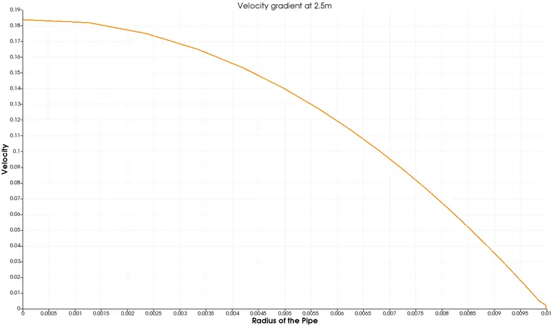
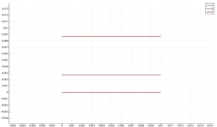
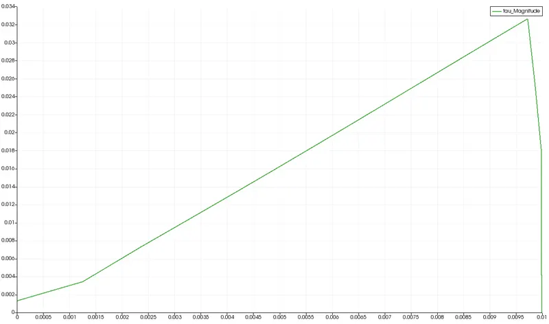
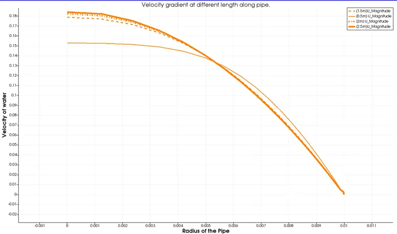
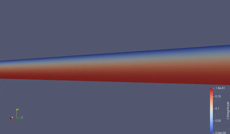
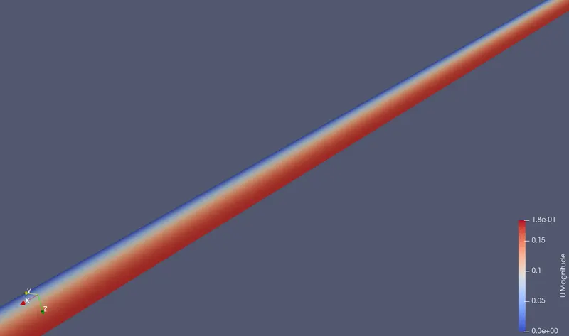
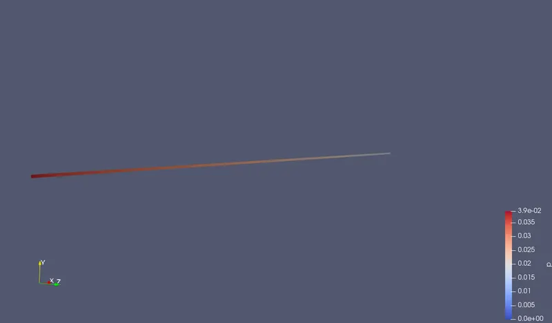
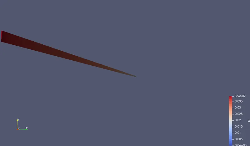
The simulation shows how the velocity and pressure will change along the length of the pipe. As we also see the shear stress accross the radius of the wedge. The variations of velocity shows that the fluid(water) is reaching the steady state as it approaches the outlet. The precise location is 2.1m from origin as it is the entrance length of the pipe.
Furthermore, as The comparision shows that there is indeed the unsteadyness which occurs due to the entrance. The shear distribution shows that there is a larger magnitude of shear at the wall (Which is obvious because of boundary condition phenomenon(no slip)).
10) Conclusion:
It is hence proven that the pressure difference governed by the Hagen-Poiseuille's equation is valid in the simulation. And provides as complete understanding of the flow inside the pipe.