Week 5 - Rayleigh Taylor Instability
|
Content
|
Aim: To understand Rayleigh-Taylor instability and to simulate it using software(Ansys Fluent).
1) Introduction:
Rayleigh Taylor instability is caused when 2 fluids of differing densities are present in a domain, a small disturbance leads to the instability. The linearity of the instability occuring is given by Atwood number.
The small disturbance creates an ever increaing pressure gradient and density gradient which increases the acceleration of instability. Also, te presence of gravity influences the gradients.
There are various forms of instabilities that occur dur the interaction between fluid of different densities.
Such as:
1) Kelvin-Helmholtz instability: These occure when there is a relative motion between 2 fluids of different densities over one another. This cause small distrubances which creates an ever increasing pressure difference and leads to swirling shaped and the instablilty occurs.
 |
Mathmatically expressed in the form of : 
also known as Taylor-Goldstein equation.
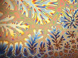
2) Saffman-Taylor instability: This is the inverse of Rayleigh-Taylor instability, where a less viscous fluid is injected into fluid with higher viscosity. The high viscous fluid is displaces leaving finger like structures.
There exist other types of instabilities as well which are slight variations of Rayleigh-Taylor instability.
 |
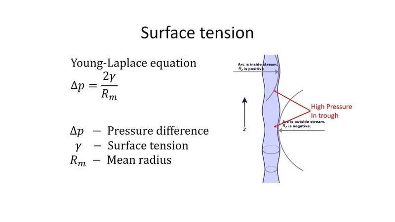
3) Plateau-Rayleigh instability: It explains why and how a falling stream of fluid breaks up into smaller packets with the same volume but less surface area.
Example a falling drop of water from a tap.
 |
In practice these type of phenomenon occure and can be simulated using CFD. For Example, simulation of mixing of air and fuel in combstion chamber, simulation of cloud formation are some of the instabilites in naturel and engineering life. These solvers for vof can be levraged to optimize the processes and problem solving.
Rayleigh-Taylor instability also provides a good understanding of stability inside a system where there is presence of multiple fluids. Small petrubations ccause major changes and the understangind of this can help in solving real life problems. It can also help in minimizing the instability.
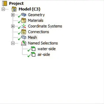
2) Problem setup in Ansys workbench
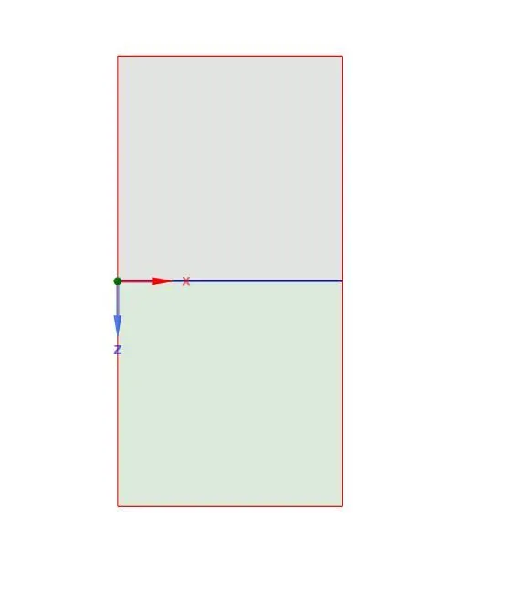
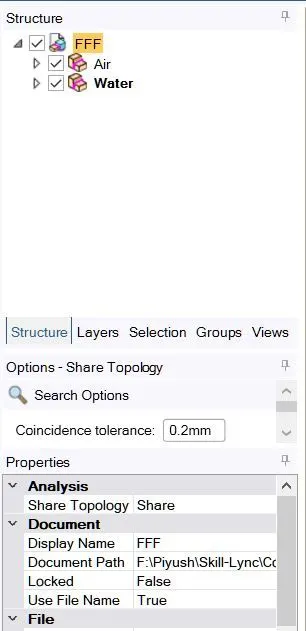
1) Geometry:
 |
 |
2) Meshing:
|
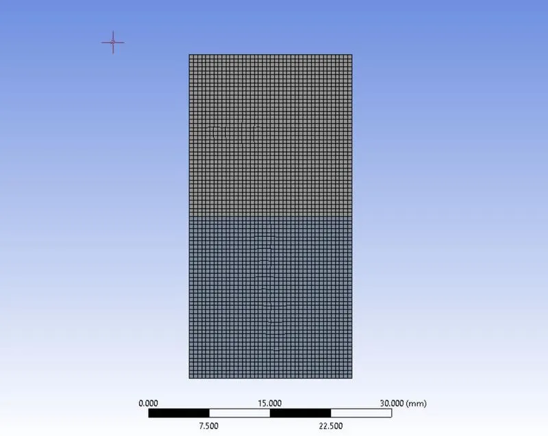
Baseline mesh- 0.5mm
|
|
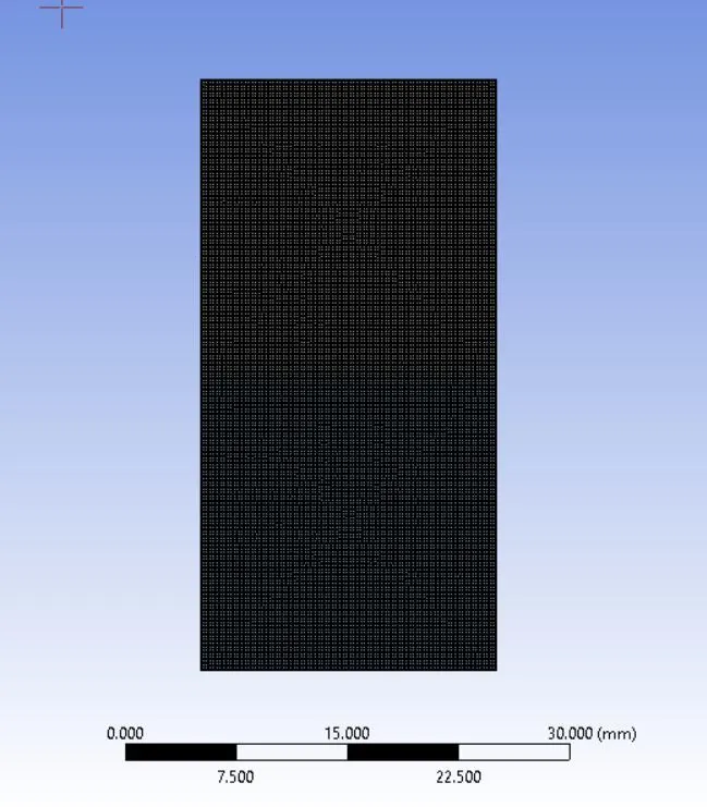
Refined mesh- 0.15mm
|
|
|
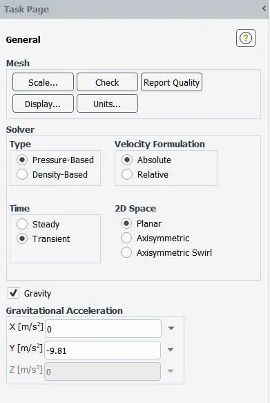
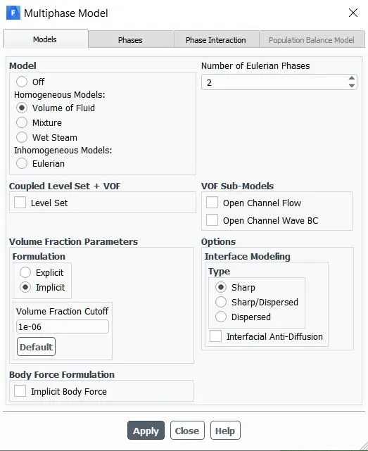
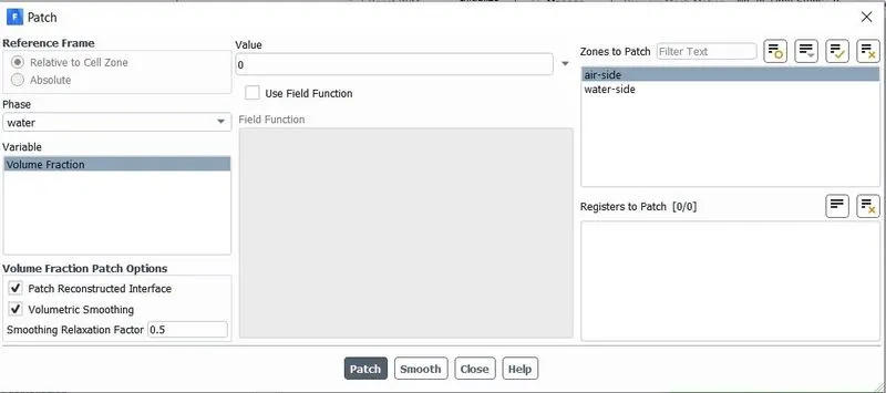
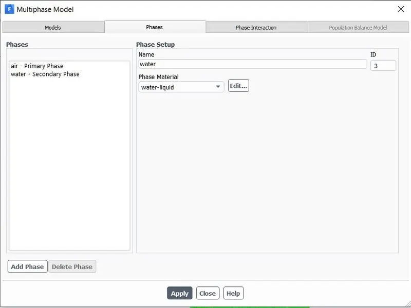
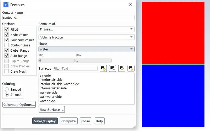
3) Setup:(Important changes in setup, rest all is default)
 |
 |
 |
 |
|
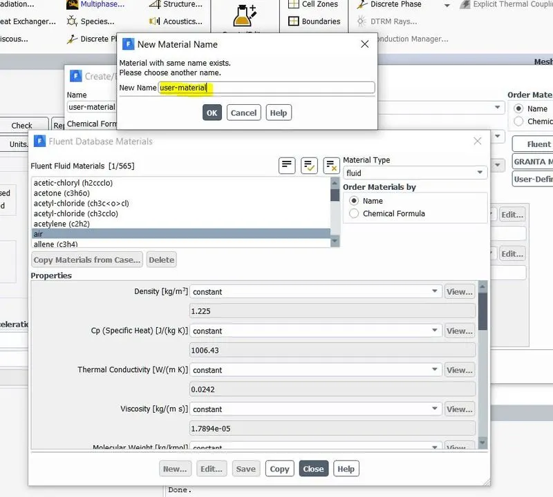
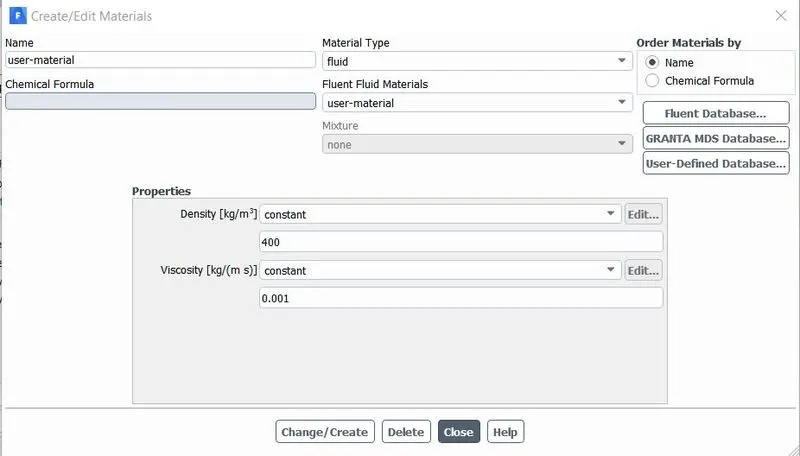
Setup for user defined material:
|
|
|
 |
3) Result:
|
1) Baseline: Drive:Baseline animation |
|
2) Refined: Drive:Refined mesh 0.15mm |
|
3) Use-Defined material: Drive:User-defined-Material |
4) Why Transient solver?
As we are concerned with the mixing of 2 fluids we want so observ how these fluids interact and how the instability is initiated. Transient solver hels us resolve this by provinding timesteps and how long we want to silulate for. As for stead state is concerned, when the fluid of higher density reaches the bottom and completely switch places wit lower density fluid, we conclude its a steady state. But as we want to see the instability we choose a transient solver.
5) Atwood number:
It is a dimentional less number which compare the densities of fluid in this kind of senario.
Atwood number is given by: `A = (rho1-rho2)/(rho1+rho2)`
From the problem statement above for the 2 cases we can evaluate Atwood number using the expression.
such as,
Case 1)
Density of water = 998.2 `(kg)/m^3`
Density of air = 1.225 `(kg)/m^3`
A = `(99802-1.225)/(998.2+1.225)` = 0.997548
Case 2)
Density of user defined material = 400`(kg)/m^3`
Density of water = 998.2 `(kg)/m^3`
A = `(998.2-400)/(400+998.2)` = 0.42783
6) Conclusion:
1) From the results above we can observe the difference between the animation of baseline(0.5mm) mesh and Refined(0.15mm)mesh. It is clear that sue to bigger elemet size there is loss of resolution in the animation. Hence, "smudging" can be seen, this is due to diffussion. This is bad as the fluid needs to mantain its density. To tackel this we make a finer mesh, the finer mesh gives result that is better in resolution and with minimal diffussion.
2) As for the Atwood number closer to 1 the larger bubble are formed i.e the lighter fluid penetrates further into the heavy fluid. The Atwood number also shows the acceleration of the heavier fluid as the instability devlopes. The fluid with reletively larger Atwood number shows a faster rate of descent into the lighter fluid than the second case. Although, the difference between the Atwood number of both cases is very small, the difference in the simulation is observable.
Hence, we can conclude that with the simulation counducted we get a good idea about the Rayleigh-Taylor instability and the influence of Atwood number on the fluids involved.