Simulation of a 1D Super-sonic nozzle flow simulation using Mac-Cormack Method
Content
|
| ----------------------------------------------------------------------------- |
A finite control volume gives us a good idea of overall understanding of the continuum and overall physics of fluid flow. When it comes to Computational Fluid Dynamics it is necessary to understand flow in 2 cases. Non-Conservation form and Conservation form. Although in analytical Fluid mechanics it does not matter how the control volume flows, in CFD it makes a substantial difference.
1) Finite Control Volume:
A control volume is a element or a space occupied by fluid which is used to analyayse the fluid element that is occupied by control volume.
There are 2 main methods to assess this behaviour of fluid inside the control volume.
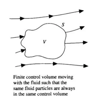
1.1) Non-Conservative:
Non-conservative form gives the inforation about the fluid flow contained inside a Control Volume whilst the Contro Volume is moving inside the continum.
This means the fluid contained inside the CV will not change, Although it's properties will and most definatily change wrt time.
 |
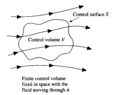
1.2) Conservative:
Conservative form defines a control volume in space through which fluid flows. The fluid flows as the CV is stationary, as the fluid changes so does the properties of the fluid and the Control Volume.
 |
As it is important to understand the behavious of fluid in fixed and moving Control Volume. It is also necessary to understand the way to convert the governing equation into a propper form and used them to create a pipeline and deploy a programm that could solve the problem(1D Converging-Diverging Nozzle in this case.)
MacCormac method: A predictor - corrector method which employs forward difference and backward difference together that gives a Secon Order Accuracy and has less computation cost compared to a normal Second order acuurate method.
We will understand this method by using a case of Convergent-Divergent nozzle in a quas-1D setting.
2) Case Setup for a 1D Convergenrt - Divergent Nozzle:
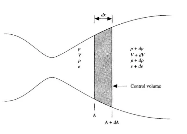 |
A convergent-divergent Nozzle is a structure that has a constantly changind cross-sectional diameter. i.e it decreases to a certain point and then it increases.
The region of least Cross-sectional area is called a throat.
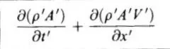
The flow is governed by equations that would predict the Density, Presseure, Velocity, Temperature (energy) through the Nozzle and at any point in time.
the equations are:
| Governing Equation | Non-Conservative | Conservative |
| Continuity | 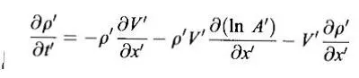 |
 |
| Momentum | 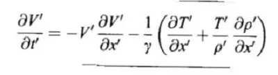 |
 |
|
Energy (Temperature) |
 |
 |
These Governing equations would give all the information about the fluid flow in both forms. Plus they predict exact physics of the flow.
The next step is to discrityze the equations according to the MacCormak Method. Although the way we discrityze the equations is different for both forms simply because of the existance of variables and theirositions inside the differential equation.
Here we will try to explain the general method of the MacCormak method and see how it is different for Consevative form.
| ----------------------------------------------------------------------------- |
A Non - Conservative Form
Nozzle geometry is given as: `A = 1 + 2.2*(x - 1.5)^2 <= x <=3`
2.1) Predictor step: In this step the Governing equations are discrityze as would any other equation,
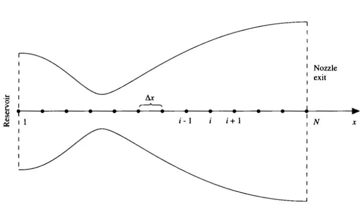
As from the above diagram discretyzation is made along the length of Nozzle.
| Discrityzed equation | |
| Continuity |  |
| Momentum |  |
| Temperature(Energy) | |
As the above equations are for a current time step and a forward difference methods is uned we can now proceed to further step where we find the primitive variables for the predictor step.
Using:
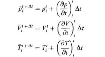 |
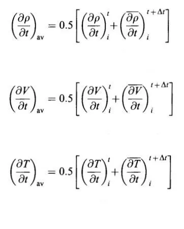
this gives us primitive variables that will be used in Corrector step where the same algebric equation is solved using the Backward Difference method.
further more the values obtained are averaged as:
 |
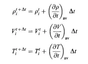
2.2) Corrected values using Corrector step:
using this we will obtain the corrected values of primitive variables which is given by:
These steps will be repeted as long as the steady state is achieved or the simulation time assigned.
2.3) Points to consider:
a) Calculating the time step: As time step and the space step is crucial for stability it is necessary to calculate the timestep that is most appropriate for maintaining the stability for the solution. As the CFL criteria is important aspect to consider we assume the Courant number to be 0.5 and using its definition we come up with, `trianglet = C*(trianglex)/(a + V)` time steps.
Where,
a = Sonic speed.
V = flow speed.
b) Boundary Conditions:Assigining Boundary conditions to the inlet and outlet is crucial for flow to occur, These boundary conditions are obtained using linear interpolation. Using the understanding of Method of Characterstics one can understand which boundary conditions are necessay and which ones need to be floated (Velocity in our case).
Inlet:(Fixed values)
`rho(1) = 1`
`t(1) = 1`
Outlet:(as per solution)
V(n) = 2V(n-1) - V(n-2)
p(n) = 2p(n-1) - P(n-2)
t(n)= 2T(n-1) - T(n-2)
| ----------------------------------------------------------------------------- |
B Conservative Form
Conservative form is one where the cotrol volume stays stationary. Asthis gives enough insight to flow the governing equation changes a bit and can be seen why.
As the CV is still the properties of fluid will change wrt time and space. Unlike the Non-Conservative form where the primitive variable are responsible for the change in shape of its CV, in Conservative formthe CV stays the same and the change in properties/Primitive values(of fluid) is observed inside the CV and they have no influence on the CV nor other way round.
Here we will see how the different representation in governing equation will affect the algebric form.
As it would be difficult to represent the variables inside the differential equations new function are created that are given as:
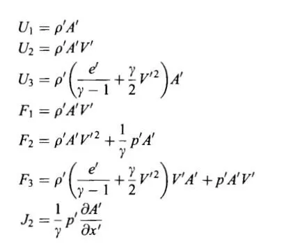
In a nutshell: we convert the Conservative form into a Non-Conservative form using variables assigned and after calculations are completer we convert them back to primitive variables.
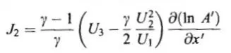
Now the governing equation can be written as:
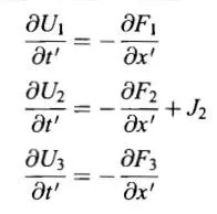
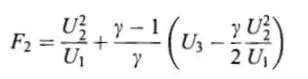
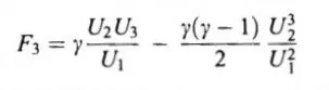
and the F1, F2, F3(Flux terms) can be discrityzed using MacCormak method.
 |
 |
 |
 |
Further the steps follow in the same way as the Non-Conservative method untilthe conver sion of U1,U2, U3 back into the primitive variable which can easily be done using the manipulation of the U1,U2, U3 equations.
3) Points to consider.
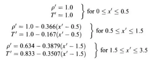
Initial Condition:
Boundary Conditions:
U1 = A(1) = fixed value
U2 = 2*U2(2) - U2(3)
`U3 = U1*(t/(gamma -1)+(gamma/2)*v^2)`
Time step is calculated according to the pervious step.
This marks the end of theory of the various aspects of simulation,the math, physics behind it.
| ----------------------------------------------------------------------------- |
4)
As we have seen from the theory we will try to simulate the process using MATLAB code.
4.1) Non-Conservative form:
%Non-Conservative form function

function [rho, t, v, p, M, rho_th, v_th, p_th, t_th, M_th, mfr, mfr_th] = main_prog(n, x, dx, g)


    %calculating initial profiles
    rho = 1-0.3146*x;
    t = 1-0.2314*x; %t = temperature
    v = (0.1+1.03*x).*t.^0.5;
    M = zeros(1, n);

    %area
    a = 1+2.2*(x-1.5).^2;
    th = find(a==min(a));    %Throat area

    %Time steps
    nt = 1400;  %Time steps
    C = 0.5;    %Courant number
    dt_g = C*(dx./((t.^0.5)+v)); %CFL criteria
    dt = min(dt_g);  %Time step

    %Time loop
    for k=1:nt
        %Copying the Variable
        rho_old = rho;
        v_old = v;
        t_old = t;

        %Predictor method
        for j = 2:n-1 %inner loop

            dvdx = (v(j+1)-v(j))/dx;
            drhodx = (rho(j+1)-rho(j))/dx;
            dtdx = (t(j+1)-t(j))/dx;
            dlogadx = (log(a(j+1))-log(a(j)))/dx;

            %Continuity equation
            drhodt_p(j) = -rho(j)*dvdx -rho(j)*v(j)*dlogadx -v(j)*drhodx;

            %Momentum equation
            dvdt_p(j) = -v(j)*dvdx-(1/g)*(dtdx + (t(j)/rho(j))*drhodx);

            %Energy equation
            dtdt_p(j) = -v(j)*dtdx -(g-1)*t(j)*(dvdx + v(j)*dlogadx);

            %Solution update
            rho(j) = rho(j) + drhodt_p(j)*dt;
            v(j) = v(j) + dvdt_p(j)*dt;
            t(j) = t(j) + dtdt_p(j)*dt;
        end

        %Corrector method
        for j = 2:n-1 %inner loop
            dvdx = (v(j)-v(j-1))/dx;
            drhodx = (rho(j)-rho(j-1))/dx;
            dtdx = (t(j)-t(j-1))/dx;
            dlogadx = (log(a(j))-log(a(j-1)))/dx;

            %Continuity equation
            drhodt_c(j) = -rho(j)*dvdx -rho(j)*v(j)*dlogadx -v(j)*drhodx;

            %Momentum equation
            dvdt_c(j) = -v(j)*dvdx-(1/g)*(dtdx + (t(j)/rho(j))*drhodx);

            %Energy equation
            dtdt_c(j) = -v(j)*dtdx -(g-1)*t(j)*(dvdx + v(j)*dlogadx);


        end

        %Compute average time derivative

        drhodt = 0.5*(drhodt_p + drhodt_c);
        dvdt = 0.5*(dvdt_p + dvdt_c);
        dtdt = 0.5*(dtdt_p + dtdt_c);

        %final solution update

        for i = 2:n-1
            rho(i) = rho_old(i) + drhodt(i)*dt;
            v(i) = v_old(i) + dvdt(i)*dt;
            t(i) = t_old(i) + dtdt(i)*dt;
        end

        %apply boundary condition

        %inlet
        v(1) = 2*v(2) - v(3);

        %outlet
        v(n) = 2*v(n-1) - v(n-2);                %velocity
        rho(n) = 2*rho(n-1) - rho(n-2);          %Density
        t(n) = 2*t(n-1) - t(n-2);                %temperature

        p = rho.*t;                              %Pressure
        M = v./(t.^0.5);                         %Mach number
        mfr = rho.*a.*v;                         %Mass Flow rate

        %Calculating values at throat
        rho_th(k) = rho(th);
        v_th(k) = v(th);
        t_th(k) = t(th);
        p_th(k) = p(th);
        M_th(k) = M(th);
        mfr_th(k) = mfr(th);

        figure(1)
        %Mass flow rate along the nozzle length for perticular timesteps
        grid on
        title("Variation of Mass flow rate at different timestep")
        xlabel("Nozzle Length")
        ylabel("Mass flow rate at Specific Iteration")
        if k==200
            plot(x, mfr)
            hold on
        elseif k == 400
            plot(x, mfr)
            hold on

        elseif k == 700
            plot(x, mfr)
            hold on
        elseif k == 900
            plot(x, mfr)
            hold on
        elseif k == 1200
            plot(x, mfr)
            hold on
        elseif k ==1400
            plot(x, mfr, 'linewidth', 1.5)

            legend("Time step: 200","Time step: 400", "Time step: 700","Time step: 900", "Time step: 1200", "Time step: 1400" )

        end
    end

end
4.2) Conservative form:
%Conservative Form
%the function gives the primitive values as arraays in the output which
%will give a plot that is requaired.

function [rho_c, t_c, v_c, p_c, M_c, rho_th_c, v_th_c, p_th_c, M_th_c, t_th_c, mfr_c, mfr_th_c] = c_conservative(n, x, dx, g)

    %Initial conditions
    for i = 1:n
        if (x(i) >= 0) && (x(i) <= 0.5)
            rho_c(i) = 1;
            t_c(i) = 1;

        elseif (x(i) >= 0.5) && (x(i) <= 1.5)
            rho_c(i) = 1 - 0.366*(x(i) - 0.5);
            t_c(i) = 1 - 0.167*(x(i) - 0.5);

        elseif (x(i) >= 1.5) && (x(i) <= 3)
            rho_c(i) = 0.634 - 0.3879*(x(i) - 1.5);
            t_c(i) = 0.833 - 0.3507*(x(i) - 1.5);
        end
    end
    a = 1+2.2*(x-1.5).^2;   %Area
    th = find(a==min(a));   %Throat area

    v_c = (0.59)./(rho_c.*a); %velocity


    %Assigining a zero vectors for solution vectors
    U1 = rho_c .* a;
    U2 = rho_c.*v_c.*a;
    U3 = rho_c.*a.*((t_c./(g-1)) + (g/2).*(v_c.^2));


    C = 0.5; %Courant  number

    dt_t = C*(dx./(t_c.^0.5+v_c));
    nt = 1400;
    dt = min(dt_t);

    %Timesteps/ loop
    for o = 1:nt
        U1_old = U1;
        U2_old = U2;
        U3_old = U3;

        %Flux vectors
        F1 = U2;
        F2 = (U2.^2./U1) + ((g-1)/g)*(U3 - (g*0.5*U2.^2./U1));
        F3 = (g*U2.*U3./U1) - (g*(g-1)*0.5)*(U2.^3./U1.^2);

        %Predictor method
        for p = 2:n-1
            J2 = (1/g)*rho_c.*t_c.*((a(p+1) - a(p))/dx);
             %continuity equation
             dU1dx_p(p) = -((F1(p+1)-F1(p))/dx);

             %Momentum equation
             dU2dx_p(p) = -((F2(p+1)-F2(p))/dx) + J2(p);

             %Energy equation
             dU3dx_p(p) = -((F3(p+1)-F3(p))/dx);

             %updating the soulution vectors
             U1(p) = U1(p)+dU1dx_p(p)*dt;
             U2(p) = U2(p)+dU2dx_p(p)*dt;
             U3(p) = U3(p)+dU3dx_p(p)*dt;


        end

        %Updating the primitive values
         rho_c = U1./a;
         t_c = (g-1)*(U3./U1 - (g/2)*(U2./U1).^2);


        %Calculating Flux vectors using predicted values
        F1_p = U2;
        F2_p = (U2.^2./U1) + ((g-1)/g)*(U3 - (g*0.5*U2.^2./U1));
        F3_p = (g*U2.*U3./U1) - (g*(g-1)*0.5)*(U2.^3./U1.^2);

        %Corrector step
        for c =2:n-1
            J2_p = (1/g)*rho_c.*t_c.*((a(c) - a(c-1))/dx);

            %Continuity equation
            dU1dx_c(c) = -((F1_p(c) - F1_p(c-1))/dx);

            %Momentum Equation
            dU2dx_c(c) = -((F2_p(c) - F2_p(c-1))/dx) + J2_p(c);

            %Energy equation
            dU3dx_c(c) = -((F3_p(c) - F3_p(c-1))/dx);


        end

        %Averaged values of predictor and corrector steps.
        dU1dx_av = 0.5*(dU1dx_p + dU1dx_c);
        dU2dx_av = 0.5*(dU2dx_p + dU2dx_c);
        dU3dx_av = 0.5*(dU3dx_p + dU3dx_c);

        %Final updated values of solution vector for oth time step.
        for q = 2:n-1
            U1(q) = U1_old(q) + dU1dx_av(q)*dt;
            U2(q) = U2_old(q) + dU2dx_av(q)*dt;
            U3(q) = U3_old(q) + dU3dx_av(q)*dt;
        end

        %Boundary Conditions
        %Inlet
        U1(1) = rho_c(1)*a(1);
        U2(1) = 2*U2(2) - U2(3);
        v_c(1) = U2(1)./U1(1);
        U3(1) = U1(1)*((t_c(1)/(g-1)) + (g*0.5*(v_c(1))^2));

        %Oulet
        U1(end) = 2*U1(end-1) - U1(end-2);
        U2(end) = 2*U2(end-1) - U2(end-2);
        U3(end) = 2*U3(end-1) - U3(end-2);

        %Calculating the primitive variables using the final solution
        %vector
        rho_c = U1./a;
        v_c = U2./U1;
        t_c = (g-1)*((U3./U1) - (g*0.5)*(v_c).^2);

        p_c = rho_c .* t_c;
        M_c = v_c ./ (sqrt(t_c));
        mfr_c = rho_c.* a .* v_c;

        %Computing primitive variables at the throat section.
        rho_th_c(o) = rho_c(th);
        p_th_c(o) = p_c(th);
        M_th_c(o) = M_c(th);
        t_th_c(o) = t_c(th);
        v_th_c(o) = v_c(th);
        mfr_th_c(o) = mfr_c(th);


        figure(4)
        %Mass flow rate accross the Nozzle for perticulat time steps.
        title("Variation of Mass flow rate at different timestep")
        xlabel("Nozzle Length")
        ylabel("Mass flow rate at Specific Iteration")
        grid on

        if o == 200
            plot(x, mfr_c)
            hold on
        elseif o == 400
            plot(x, mfr_c)
            hold on
        elseif o ==700
            plot(x, mfr_c)
            hold on
        elseif o == 1000
            plot(x, mfr_c)
            hold on
        elseif o ==1200
            plot(x, mfr_c)
            hold on
        elseif o == 1400
            plot(x, mfr_c, 'linewidth', 1.5)
            hold on
            legend("Time step: 200","Time step: 400", "Time step: 700","Time step: 900", "Time step: 1200", "Time step: 1400" )

        end

    end


end
4.3) Plotting:
close all
clear all
clc

n = 31;
x = linspace(0, 3, n);
dx = x(2)-x(1);
g = 1.4;
nt = 1400;

prp = "choose your form: ";
r = input(prp);

if r == 1
    %Non-Conservative Form
    [rho, t, v, p, M, rho_th, v_th, p_th, t_th, M_th, mfr, mfr_th] = main_prog(n, x, dx, g);

    figure(2)
    %Plotiing the time wise variation for variables
    subplot(4, 1, 1)
    plot(linspace(1, nt, nt), rho_th,'color', 'm')
    ylabel("Density")
    title("Time-wise variation of variables")

    subplot(4, 1, 2)
    plot(linspace(1, nt, nt), t_th, 'color', 'r')
    ylabel("Temperature")

    subplot(4, 1, 3)
    plot(linspace(1, nt, nt), p_th, 'color', 'y')
    ylabel("Pressure")

    subplot(4, 1, 4)
    plot(linspace(1, nt, nt), M_th, 'color', 'c')
    ylabel("Mach no.")
    xlabel("Time-steps")


    figure(3)
    %Properties varying along the length of Nozzle
    subplot(4, 1, 1)
    plot(x, rho, 'color', 'm')
    ylabel("Density")
    title("Variation of variables along length of Nozzle")

    subplot(4, 1, 2)
    plot(x, p, 'color', 'r')
    ylabel("Pressure")

    subplot(4, 1, 3)
    plot(x, t, 'color', 'y')
    ylabel("Temperature")

    subplot(4, 1, 4)
    plot(x, M, 'color', 'c')
    ylabel("Mach no.")
    xlabel("Length of Nozzle")


elseif r == 2
    %Conservative form
    [rho_c, t_c, v_c, p_c, M_c, rho_th_c, v_th_c, p_th_c, M_th_c, t_th_c, mfr_c, mfr_th_c] = c_conservative(n, x, dx, g);

    figure(5)
    %Plotiing the time wise variation for variables
    subplot(4, 1, 1)
    plot(linspace(1, nt, nt), rho_th_c, 'color', 'm')
    ylabel("Density")
    title("Time-wise variation of variables")

    subplot(4, 1, 2)
    plot(linspace(1, nt, nt), t_th_c, 'color', 'r')
    ylabel("Temperature")

    subplot(4, 1, 3)
    plot(linspace(1, nt, nt), p_th_c, 'color', 'y')
    ylabel("Pressure")

    subplot(4, 1, 4)
    plot(linspace(1, nt, nt), M_th_c, 'color', 'c')
    ylabel("Mach no.")
    xlabel("Time-steps")


    figure(6)
    %Lenght wise variation of primitive variables
    subplot(4, 1, 1)
    plot(x, rho_c, 'color', 'm')
    ylabel("Density")
    title("Variation of variables along length of Nozzle")

    subplot(4, 1, 2)
    plot(x, p_c, 'color', 'r')
    ylabel("Pressure")

    subplot(4, 1, 3)
    plot(x, t_c, 'color', 'y')
    ylabel("Temperature")

    subplot(4, 1, 4)
    plot(x, M_c, 'color', 'c')
    ylabel("Mach no.")
    xlabel("Length of Nozzle")

elseif  r == 3
    %Comparision of mass flow rate of Non-conservative form vs Conservative
    %form.
    [rho, t, v, p, M, rho_th, v_th, p_th, t_th, M_th, mfr, mfr_th] = main_prog(n, x, dx, g);
    [rho_c, t_c, v_c, p_c, M_c, rho_th_c, v_th_c, p_th_c, M_th_c, t_th_c, mfr_c, mfr_th_c] = c_conservative(n, x, dx, g);

    figure(7)
    plot(x, mfr, 'linewidth', 1.5)
    hold on
    grid on
    plot(x, mfr_c, 'linewidth', 1.5)
    title('Comparision of Mass flow rate od Conservative and Non-Conservative form')
    xlabel("Length of Nozzle")
    ylabel("Mass Flow rate")
    legend("Non-conservative form", "Conservative form")

end| ----------------------------------------------------------------------------- |
5) Output:
5.1) Non-Conservative form
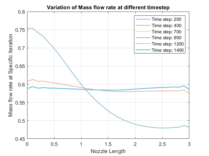
| a) Mass flow rate at perticular time steps |
 |
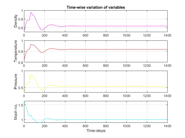
| b) Time wise variation of primitive variables |
 |
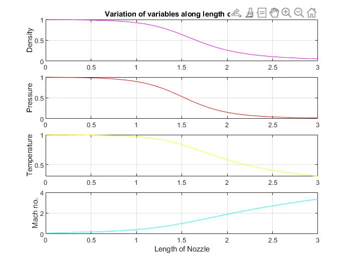
| c) Lenght wise variation of primitive variables |
 |
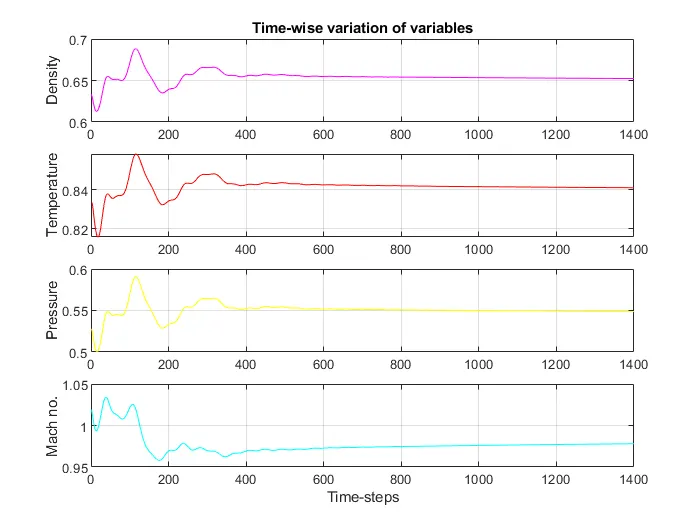
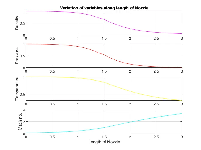
5.2) Conservative form
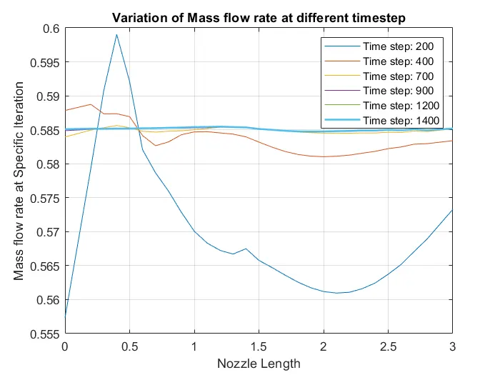
| a) Mass flow rate at a perticular time steps |
 |
| b) Time wise variation of primitive variables |
 |
| c) Length wise variation of primitive variables |
 |
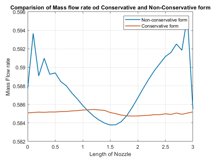
5.3) Comparision of normalised mass flow rate:
| Comparision of Normalised mass flow rate for Non-Conservative and Conservative form |
 |
| ----------------------------------------------------------------------------- |
6) Comments on the output:
At first glance it can be assumed that both the forms should be same as the caseis same for both the cases. But, it is far from the truth, as we have already seen how the Conservative form works and Non-Conservative form works w.r.t to its flow and control volume it is only obvious to know that even thought in both cases the steady state is achieved the time/ iterations taken and the general way a variable reaches its steady state differs. For example, the time wise variation of the variables show that for it to reach at a steady state Non-Conservative form required close to 400 timesteps and for Conservative form the variations are high and hence it reaches the steady state after 400th timestep.
This gives enough insight into the under standing of both forms. Eve though they reach steady state(CFL criteria), the way both forms function are different.
7) Conclusion:
Hence, we can conclude the validity of Mac-Cormak method is a second order acuurate method and can be used to do an analysis/Simulation of a quasi 1D Convergent-Divergent Nozzle.