Week 4.1 - Genetic Algorithm
Aim :-
- Write a code in MATLAB to optimise the stalagmite function and find the global maxima of the function.
- Clearly expalin the concept of genetic algorithm in your own words and also explain the syntax for ga in MATLAB in your report.
- Make sure that your code gives the same output, even if it is made to run several times.
- Plot graphs for all 3 studies and for F maximum vs no. of iterations. Title and axes labels are a must, legends could be shown if necessary
Theory :-
1. Stalagmite Function:-
A stalagmite is an upward-growing mound of mineral deposits that have precipitated from water dripping onto the floor of a cave. Most stalagmites have rounded or flattened tips.
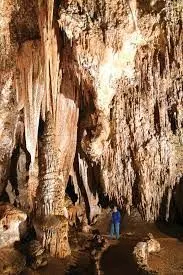
It can be traced on a graph by using a relation between mathematical relations.following mathematical model was incorporated for tracing the stalagmite model:-
`f1=(sin(5.1pix+0.5))^6`
`f2=(sin(pi y+0.5))^6`
`f3=exp[-4log(2)((x-0.0667)^2)/0.64]`
`f4=exp[-4log(2)((y-0.0667)^2)/0.64]`
`f=f1*f2*f3*f4`
2. General Algorithm:-
Genetic algorithm developed by Goldberg was inspired by Darwin's theory of evolution which states that the survival of an organism is affected by rule "the strongest species that survives". Darwin also stated that the survival of an organism can be maintained through the process of reproduction, crossover and mutation. Darwin's concept of evolution is then adapted to computational algorithm to find solution to a problem called objective function in natural fashion. A solution generated by genetic algorithm is called a chromosome, while collection of chromosome is referred as a population. A chromosome is composed from genes and its value can be either numerical, binary, symbols or characters depending on the problem want to be solved. These chromosomes will undergo a process called fitness function to measure the suitability of solution generated by GA with problem. Some chromosomes in population will mate through process called crossover thus producing new
chromosomes named offspring which its genes composition are the combination of their parent. In a generation, a few chromosomes will also mutation in their gene. The number of chromosomes which will undergo crossover and mutation is controlled by crossover rate and mutation rate value. Chromosome in the population that will maintain for the next generation
will be selected based on Darwinian evolution rule, the chromosome which has higher fitness value will have greater probability of being selected again in the next generation. After several generations, the chromosome value will converges to a certain value which is the best solution for the problem.
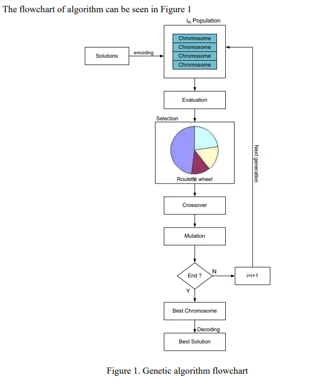
The Algorithm
In the genetic algorithm process is as follows:
Step 1. Determine the number of chromosomes, generation, and mutation rate and crossover
rate value
Step 2. Generate chromosome-chromosome number of the population, and the initialization
value of the genes chromosome-chromosome with a random value
Step 3. Process steps 4-7 until the number of generations is met
Step 4. Evaluation of fitness value of chromosomes by calculating objective function
Step 5. Chromosomes selection
Step 6. Crossover
Step 7. Mutation
Step 8. Solution (Best Chromosomes)
3. Syntax for GA:-
1. x = ga(fun,nvars)-finds a local unconstrained minimum, x, to the objective function, fun. nvars is the dimension (number of design variables) of fun.2. x = ga(fun,nvars,A,b)- finds a local minimum x to fun, subject to the linear inequalities A*x ≤ b. ga evaluates the matrix product A*x as if x is transposed (A*x').3. x = ga(fun,nvars,A,b,Aeq,beq)- finds a local minimum x to fun, subject to the linear equalities Aeq*x = beq and A*x ≤ b. (Set A=[] and b=[] if no linear inequalities exist.) ga evaluates the matrix product Aeq*x as if x is transposed (Aeq*x').4. x = ga(fun,nvars,A,b,Aeq,beq,lb,ub)-defines a set of lower and upper bounds on the design variables, x, so that a solution is found in the range lb ≤ x ≤ ub. (Set Aeq=[] and beq=[] if no linear equalities exist.)5. x = ga(fun,nvars,A,b,Aeq,beq,lb,ub,nonlcon)-subjects the minimization to the constraints defined in nonlcon. The function nonlcon accepts x and returns vectors C and Ceq, representing the nonlinear inequalities and equalities respectively. ga minimizes the fun such that C(x) ≤ 0 and Ceq(x) = 0. (Set lb=[] and ub=[] if no bounds exist.)x = ga(fun,nvars,A,b,Aeq,beq,lb,ub,nonlcon,options)-minimizes with the default optimization parameters replaced by values in options. (Set nonlcon=[] if no nonlinear constraints exist.) Create options using optimoptions.7. x = ga(fun,nvars,A,b,Aeq,beq,lb,ub,nonlcon,intcon)-requires that the variables listed in intcon take integer values.8. x = ga(problem)- finds the minimum for problem, a structure described in problem.9. [x,fval] = ga(___)- for any previous input arguments, also returns fval, the value of the fitness function at x.10. [x,fval,exitflag,output] = ga(___)-also returns exitflag, an integer identifying the reason the algorithm terminated, and output, a structure that contains output from each generation and other information about the performance of the algorithm.11. [x,fval,exitflag,output,population,scores] = ga(___)-also returns a matrix population, whose rows are the final population, and a vector scores, the scores of the final population.Coading :-
clc
close all
clear all

%Creating the Input matrix for X and Y

x= linspace(0,0.6,150);
 y= linspace(0,0.6,150);
 [xx,yy]=meshgrid(x,y);

 %creating the Stalagmite function
 for i=1:length(xx)
     for j=1:length(yy)
     input_vector(1)=xx(i,j);
     input_vector(2)=yy(i,j);
     f(i,j)=stalg_fuc(input_vector);% always giving minimum
     end
 end
tic


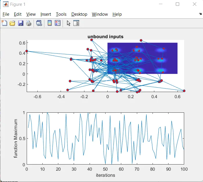
 %study1- Giving us the idea of the unbound value of stalagmite function
numcase=100;
for i=1:numcase
    [input, value(i)]=ga(@stalg_fuc,2);
    xopt(i)=input(1);
    yopt(i)=input(2);
end
Study1_time= toc
figure(1)
subplot(2,1,1)
hold on
surfc(x,y,-f)
shading interp

plot3(xopt,yopt,-value,'marker','o','markersize',5,'MarkerFaceColor','r')
title('unbound inputs')
subplot(2,1,2)
plot(-value)
xlabel('iterations')
ylabel('function Maximum')
hold off
tic
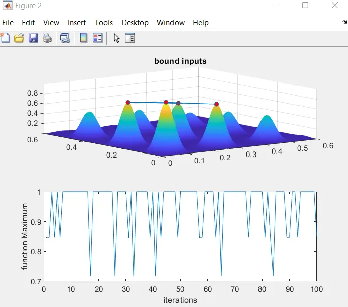
%study2- Giving us the idea of the bound value of stalagmite function

for j=1:numcase
    [input_2,fopt(j)]=ga(@stalg_fuc,2,[],[],[],[],[0;0],[0.6;0.6]);
    xopt(j)=input_2(1);
    yopt(j)=input_2(2);
end
Study2_time=toc
figure(2)
subplot(2,1,1)
surfc(xx,yy,-f)
hold on
shading interp
plot3(xopt,yopt,-fopt,'marker','o','markersize',5,'MarkerFaceColor','r')
title('bound inputs')
subplot(2,1,2)
plot(-fopt)
xlabel('iterations')
ylabel('function Maximum')
hold off

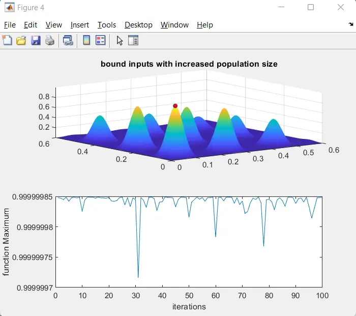
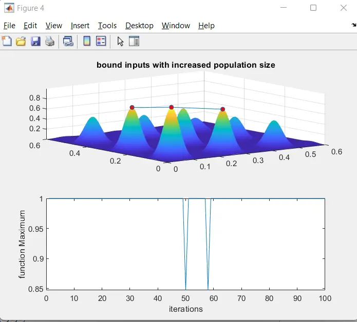
% %study 3 - Giving us the idea of the bound value of stalagmite function
% %with distinct population size
tic
 options= optimoptions('ga')
 options=optimoptions(options,'PopulationSize',400)
 for k=1:numcase
    [inputs_3, fopt(k)]= ga(@stalg_fuc, 2, [], [], [], [], [0;0],[0.6;0.6],[],[],options)
    xopt(k)=inputs_3(1);
    yopt(k)=inputs_3(2);
 end
study3_time=toc
figure(4)
subplot(2,1,1)
surfc(xx,yy,-f)
hold on
shading interp
plot3(xopt,yopt,-fopt,'marker','o','markersize',5,'MarkerFaceColor','r')
title('bound inputs with increased population size')
subplot(2,1,2)
plot(-fopt)
xlabel('iterations')
ylabel('function Maximum')
Function for Stalagmite function:-
function [f]=stalg_fuc(input)
x=input(1);
y=input(2);
f1_x=(sin(5.1*pi*(x)+0.5)).^6;
f1_y=(sin(5.1*pi*(y)+0.5)).^6;
t1=((x-0.0667).^2)./0.64;
f2_x=exp((-4.*log(2)).*t1);
t2=((y-0.0667).^2)./0.64;
f2_y=exp((-4.*log(2)).*t2);
[f]=-(f1_x.*f1_y.*f2_x.*f2_y);
end