Week 3 - Solving second order ODEs

Aim :-

write a program that solves the following ODE. This ODE represents the equation of motion of a simple pendulum with damping

In the above equation,

g = gravity in m/s2,

L = length of the pendulum in m,

m = mass of the ball in kg,

b=damping coefficient.

Write a program in Matlab\Octave that will simulate the pendulum motion, just like the one shown in the start of this challenge.

use,

L=1 metre,

m=1 kg,

b=0.05.

g=9.81 m/s2.

Theory :-

Ordinary Differential Equations

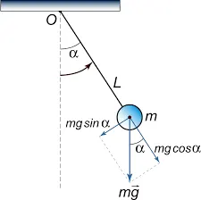
In Engineering, ODE is used to describe the transient behavior of a system. A simple example is a pendulum

The way the pendulum moves depends on the Newtons second law. When this law is written down, we get a second order Ordinary Differential Equation that describes the position of the "ball" w.r.t time.

1. Differential Equation is a mathematical equation which relates some function with its derivatives. It is important because it relates may physical laws and relation appear mathematically inthe form of such equations. It plays a prominent role in fiels such as physics, Engg, Economics and biology.

2. Differential Equation is the equation containing the derivatives of one or more dependant variable with respect to one or more independant variables. Ordinary differential equation contains a function one independant variable and its derivatives.

3. Order of a differential is the highest derivative which is present in the equation. degree is the power of highest derivative.

Dynamics of Pendulum :-

A pendulum is a weight suspended from a pivot so that it can swing freely. When a pendulum is displaced sideways from its resting, equilibrium position. The motion of the pendulum described as pe the question contains the following constants:-

g = gravity in m/s2,

L = length of the pendulum in m,

m = mass of the ball in kg,

b=damping coefficient.

Code :-

clc 
clear all
close all
%given inputs
b=0.05
g=9.81  % m/s^2
l=1     %m
m=0.1   %kg
%initial condition
theta_0=[0;3]
t_span=linspace(0,20,500)
[t, results]=ode45(@(t, theta) odefunc(t, theta, b,g,l,m), t_span, theta_0)
% Graph for output stored in the results mentioned in the above line
figure(1)
plot(t, results(:,l))
hold on
plot(t, results(:,2))
hold on
xlabel ('time')
ylabel('plot')
title('Plotting')
legend('time vs displacement', 'time vs velocity')
%Animation command for the oscilation of pendulum
ct=1;
for i=1:length(results(:,1))
    xstart=0
    ystart=0
    xend=l*sin(results(i,1))
    yend=-l*cos(results(i,1))
    
figure(2)
    plot([-1 1],[0 0], 'linewidth',5)
hold on
plot([xstart xend],[ystart yend],'linewidth',3 )% error results(:,1)
hold on
plot(xend , yend, 'o', 'markersize',20,'markerfacecolor','y' )%erroe face was not written
axis([-1.5 1.5 -2 2])
title('Pendullum Oscillation')
pause(0.0003)
hold off
k(ct)= getframe(gcf)
ct=ct+1;
end
movie(k)
videofile= VideoWriter('Oscilationpendulum.avi','Uncompressed AVI')
open(videofile)
writeVideo(videofile, k)
close(videofile)

Function Used :-

function [dtheta_dt]= odefunc(t, theta, b , g, l , m)
theta1=theta(1)
theta2=theta(2)
dtheta1_dt=theta2
dtheta2_dt=-(b/m)*theta2-(g/l)*sin(theta1)
dtheta_dt=[dtheta1_dt;dtheta2_dt]
end

Explaination :-

1. The Code should be initiated in the with the following commands:-

(a) CLC:- Clear all commands from command window.

(b)CLEAR ALL:- Clear all the work space

(c)CLOSE ALL:- Closes all the running windows in the MATLAB.

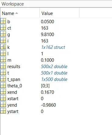
2. Next step would be to declare the initial give data for motion of pendulum. Matrix for theta for the declared with initial condition as 0 degree and velocity as 3rad/s. Time was declare with 500 intervals between 0 to 20 Sec.

3. The next step is to calculate the vlaues of angle and angular velocity for different values of time. Before the calculation we need to declare the function odefunc with parameters as (B,G,L,M, theta and t).

4. In the Function we first declare the two varibles to convert the 2nd order ODE to Linear Differential Equation. and Then as per the manipulations given below we calculate the value of angle and angular velocity:-

Theta = Theta1

DTheta1/DT= Theta2;

DTheta2/Dt=(-b/m)*(Theta20)-g/l*(Sin(Theta1))

5. After gettin the values of both the vlaues we plot then in the graph termed as PLOTTING.

6. Finally we move on with the code for presenting the motion of pendulum oscilation based on the outputs of the code which we received for the given equation.

Output :-

Graph

Output Explaination :-

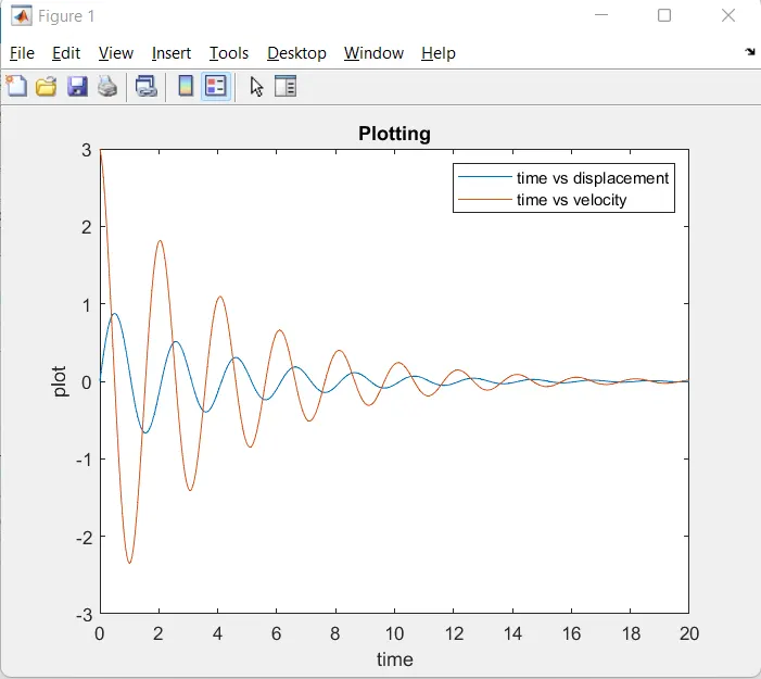
As we can see above that for the results output has 2 collumns. As it is understood that the code is returning 2 values for a single input of time one is anglular displacement other is angular velocity. And from the graph it is clear that during the initial stages of the oscillation the pendulum bob is displaced to the largest extent and then it is radually reducing to zero. It can also be seen from the graph that velocity and displacement are making 90Degree phase difference.

Youtube Link for Animation Video :-

https://youtu.be/6MD1LmHAQcs

Error Whille Coding :-

While Coding for the Animation theinput for both the angle which i have taken as Cos(:,1) and Sin(:,1)

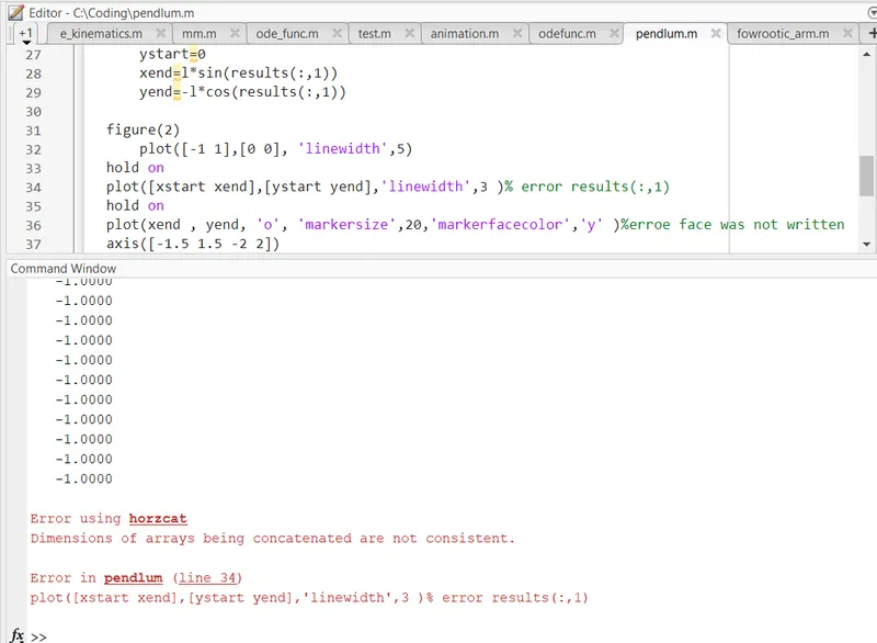
Therefore to correct it cos(i,1)&sin(i,1) was implimented an the code ran perfectly.