Week 11 - Simulation of Flow through a pipe in OpenFoam
Hagen Poiseuile flow
In this project we simulate the laminar flow through the pipe , and validate it with the analytical results by using hagen poiseulles model, Numerical results are obtained by solving in OpenFOAM , The Mesh is generated by using matlab.
Pipe is modelled as a wedge which is nothing but a sector of maximum angle of 5 deg , this code below creates a "blockMeshDict" file which takes an input of diameter , length and wedge angle
The above code creates a text file which is used to generate blockMeshDict of wedge, the output of this file
code
%% file for generating the wedge blockmesh %%
x = zeros(6,1);
x(2) = input("enter the length of the cylinder :")
x(4:5) =x(2);
y = zeros(6,1);
y(3:6) = input("enter the radius  ")
theta = input("enter the wedge angle in deg ")
z = zeros(6,1);
z(3:4) = tand(theta*0.5)*y(3);
z(5:6)= -z(3);
nx= 100;
ny =1;
nz=15;
f ="blockMeshDict.txt";
f1=fopen(f,"w");
fprintf(f1,"\n ")
fprintf(f1,"%s","FoamFile")
fprintf(f1,"\n ")
fprintf(f1,"%s","{")
fprintf(f1,"\n ")
fprintf(f1,"%s","version           2.0;")
fprintf(f1,"\n ")
fprintf(f1,"%s","format           ascii;")
fprintf(f1,"\n ")
fprintf(f1,"%s","class           dictionary;")
fprintf(f1,"\n ")
fprintf(f1,"%s","object           blockMeshDict;")
fprintf(f1,"\n ")
fprintf(f1,"%s","}")
fprintf(f1,"\n ")
fprintf(f1,"%s","convertToMeters   1;")
fprintf(f1,"\n \n \n")
fprintf(f1,"%s","vertices ");
fprintf(f1,"\n")
fprintf(f1,"%s","(")
fprintf(f1,"\n")
%x =[0 0.1 0 0.1 0.1 0];
%y =[0 0 0.05 0.05 0.05 0.05];
%z=[0 0 0.00218 0.00218 -0.00218 -0.00218];
for i = 1:length(x)
  fprintf(f1,"%s","(")
  fprintf(f1,"%d",x(i))
  fprintf(f1,"%7d",y(i))
  fprintf(f1,"%14d",z(i))
  fprintf(f1,"%s",")")
  fprintf(f1,"\n")
endfor
fprintf(f1,"%s",")")
fprintf(f1,"%s",";")
fprintf(f1, "\n \n")
fprintf(f1,"%s","blocks")
fprintf(f1, "\n")
fprintf(f1,"%s","(")
fprintf(f1, "\n \t")
fprintf(f1,"%s","hex (0 1 1 0 2 3 4 5) (")
fprintf(f1,"%d",nx)
fprintf(f1,"%3d",ny)
fprintf(f1,"%3d",nz)
fprintf(f1,"%s",") simpleGrading (1 1 1 )")
fprintf(f1, "\n")
fprintf(f1,"%s",");")
boundary = ["inlet";"outlet";"top" ;;"front";"Back";"Axis"];
b =cellstr(boundary);
faces =  ["(0 0 2 5)";"(1 1 4 3)" ;"(2 3 4 5)";"(0 1 3 2)"; "(0 1 4 5)"; "(0 1 1 0)"];
f = cellstr(faces);
type = ["type patch;";"type patch;";"type wall;" ;"type wedge;";"type symmetry;"; "type empty;"];
t =cellstr(type);
fprintf(f1,"\n \n")
fprintf(f1,"%s","edges ( ")
fprintf(f1,"\n \t")
fprintf(f1,"%s",");")
fprintf(f1,"\n \n ")
fprintf(f1,"%s","boundary ")
 fprintf(f1,"\n")
 fprintf(f1,"%s","(")
for j = 1:length(b)
fprintf(f1,"\n \n")
fprintf(f1,"%s",b{j})
fprintf(f1,"\n")
fprintf(f1,"%s","{")
fprintf(f1,"\n \t")
fprintf(f1,"%s",t{j})
fprintf(f1,"\n \t")
fprintf(f1,"%s","faces (")
fprintf(f1,"\n \t")
fprintf(f1,"%s",f{j})
fprintf(f1,"\n \t")
fprintf(f1,"%s",");")
fprintf(f1,"\n")
fprintf(f1,"%s","}")
endfor
fprintf(f1,"\n")
fprintf(f1,"%s",");")
fprintf(f1,"\n \n")
fprintf(f1,"%s","mergePatchPairs (")
fprintf(f1,"\n")
fprintf(f1,"%s",");")
fclose(f1);
output gives a blockMeshDict.txt file
 FoamFile
 {
 version           2.0;
 format           ascii;
 class           dictionary;
 object           blockMeshDict;
 }
 convertToMeters   1;


vertices
(
(0      0             0)
(2.05      0             0)
(0  0.005   0.000218305)
(2.05  0.005   0.000218305)
(2.05  0.005  -0.000218305)
(0  0.005  -0.000218305)
);

blocks
(
 	hex (0 1 1 0 2 3 4 5) (100  1 15) simpleGrading (1 1 1 )
);

edges (
 	);

 boundary
(

inlet
{
 	type patch;
 	faces (
 	(0 0 2 5)
 	);
}

outlet
{
 	type patch;
 	faces (
 	(1 1 4 3)
 	);
}

top
{
 	type wall;
 	faces (
 	(2 3 4 5)
 	);
}

front
{
 	type wedge;
 	faces (
 	(0 1 3 2)
 	);
}

Back
{
 	type symmetry;
 	faces (
 	(0 1 4 5)
 	);
}

Axis
{
 	type empty;
 	faces (
 	(0 1 1 0)
 	);
}
);

mergePatchPairs (
);
length of the cylinder is taken to 2.05 m
diameter to 0.005 m
wedge angle of 5 deg
the length is very large since we are focussing on a fully developed flow, for a fully developed flow the hydrodynamic entry length is given by
`L = 0.05*Re*D`
and the flow is laminar with
`Re =2100`
assuming a diameter 0.005 m , we get
`L =1.05 +1 ` added extra 1 for fully developed flow
considering the fully developed flow we have taken as 2.05 m
velocity calculated by using the reynolds number relation
`Re =(rho*V*D)/mu`
where `mu =1.004e-3` is the dynamic viscosity
velocity = 0.21084 m/s
calculatng the kinematic pressure at the outlet using these inputs by the hagen-Poiseuille relation
`p_2/rho =(p_1/rho)-(8*mu*l*v)/(R^2*rho`
we get "0.86114 -m2/s2"
The velocity boundary conditions in 0/U file
/*--------------------------------*- C++ -*----------------------------------*\
  =========                 |
  \\      /  F ield         | OpenFOAM: The Open Source CFD Toolbox
   \\    /   O peration     | Website:  https://openfoam.org
    \\  /    A nd           | Version:  7
     \\/     M anipulation  |
\*---------------------------------------------------------------------------*/
FoamFile
{
    version     2.0;
    format      ascii;
    class       volVectorField;
    object      U;
}
// * * * * * * * * * * * * * * * * * * * * * * * * * * * * * * * * * * * * * //

dimensions      [0 1 -1 0 0 0 0];

internalField   uniform (0 0 0);

boundaryField
{
    inlet
    {
        type            fixedValue;
        value           uniform (0.21084 0 0);
    }

    top
    {
        type                 noSlip;

    }

    Back
    {
        type            symmetry;
    }

    front
    {
        type            wedge;
    }

   outlet
   {
       type         zeroGradient;
   }

   Axis

   {
     type             empty;
   }


}


// ************************************************************************* //
The Pressure boundary conditions in 0/U file
/*--------------------------------*- C++ -*----------------------------------*\
  =========                 |
  \\      /  F ield         | OpenFOAM: The Open Source CFD Toolbox
   \\    /   O peration     | Website:  https://openfoam.org
    \\  /    A nd           | Version:  7
     \\/     M anipulation  |
\*---------------------------------------------------------------------------*/
FoamFile
{
    version     2.0;
    format      ascii;
    class       volScalarField;
    object      p;
}
// * * * * * * * * * * * * * * * * * * * * * * * * * * * * * * * * * * * * * //

dimensions      [0 2 -2 0 0 0 0];

internalField   uniform 1;

boundaryField
{

    inlet
     {

      type       zeroGradient;

     }

    outlet
      {

      type          fixedValue;
      value         uniform 0.86114;

      }

    top
    {
        type            zeroGradient;
    }

    front
    {
        type            wedge;
    }

   Back

   {

    type              symmetry;


  }

    Axis

 {
     type               empty;

   }

}

// ************************************************************************* //
The transport properties is the kinematic viscosity which is substitued in the constan/transportProperties
/*--------------------------------*- C++ -*----------------------------------*\
  =========                 |
  \\      /  F ield         | OpenFOAM: The Open Source CFD Toolbox
   \\    /   O peration     | Website:  https://openfoam.org
    \\  /    A nd           | Version:  7
     \\/     M anipulation  |
\*---------------------------------------------------------------------------*/
FoamFile
{
    version     2.0;
    format      ascii;
    class       dictionary;
    location    "constant";
    object      transportProperties;
}
// * * * * * * * * * * * * * * * * * * * * * * * * * * * * * * * * * * * * * //

nu              [0 2 -1 0 0 0 0] 1.004e-6;


// ************************************************************************* //
The laminar pipe is solved from 5 sec,the control dict file
/*--------------------------------*- C++ -*----------------------------------*\
  =========                 |
  \\      /  F ield         | OpenFOAM: The Open Source CFD Toolbox
   \\    /   O peration     | Website:  https://openfoam.org
    \\  /    A nd           | Version:  7
     \\/     M anipulation  |
\*---------------------------------------------------------------------------*/
FoamFile
{
    version     2.0;
    format      ascii;
    class       dictionary;
    location    "system";
    object      controlDict;
}
// * * * * * * * * * * * * * * * * * * * * * * * * * * * * * * * * * * * * * //

application     icoFoam;

startFrom       latestTime;

startTime       0;

stopAt          endTime;

endTime         5;

deltaT          0.0001;

writeControl    timeStep;

writeInterval   100;

purgeWrite      0;

writeFormat     ascii;

writePrecision  6;

writeCompression off;

timeFormat      general;

timePrecision   6;

runTimeModifiable true;


// ************************************************************************* //
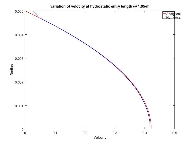
IcoFoam solver for 5 seconds, for time step 0.001 the validation of numerical and analytical results at Hydrostatic entry length
maximum velocity in numerical 0.41339 ;maximum velocity in analytical 0.42186, and the % variation is 2%
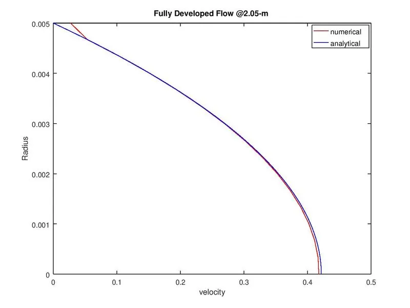
The validation with analytical solution at fully developed flow , at a length of 2.05 m
where the maximum velocity in numerical result is 0.41786, and maximum velocity in analytical result is 0.42168;
The % change in variation is 0.9%
Pressure variation in length
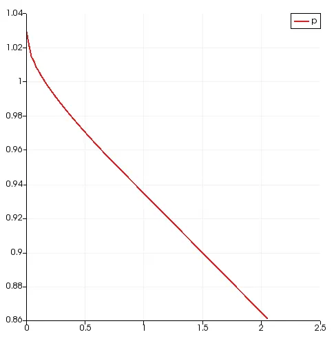
The pressure drop in the analytical case in fully developed flow is 0.138, where as in the case of numerical case 0.168
The shear stress in calculated by using the newton's law of viscosity , for newtonian fluids
`tau=mu*((du)/dy)`
in the analytical case `tau_(analytical)=0.846 N/(m^2)`
in the numerical case `tau_(Numerical)=0.83906 -N/(m^2`