Week 6 - Multivariate Newton Rhapson Solver

ODE : Ordinary differential equation

MVNR : multi variate newton raphson method

FDS: forward difference scheme

Aim : To find the roots of the first order 3 -ODE by using the multi variate newton raphson method

Methodology: To apply the MVNR , for a system of 3 ODE's , we convert into an implicit form by using the FDS .

`dy_1/(dt) = -0.04y_1 +10^4y_2y_3`

`dy_2/(dt) = 0.04y_1 -10^4y_2y_3-3*10^7y_2^2`

`dy_3/(dt) = 3*10^7y_2^2`

Conversion of the above equation into implicit forms

`dy_1/(dt) = (y_1^(n+1) -y_1^(n))/(Deltat) =-0.04y_1 +10^4y_2y_3`

`y_1^(n+1) = y_1^(n) -0.04y_1*(Deltat) +10^4y_2y_3*(Deltat)`

similary for the other two equations

`y_2^(n+1) = y_2^(n) +0.04y_1*(Deltat) -10^4y_2y_3*(Deltat)-3*10^7y_2^2*(Deltat)`

`y_3^(n+1) = y_3^(n) +3*10^7y_2^2*(Deltat)`

These equations are converted into MVNR method in the below form , where `alpha` is the relaxation factor , the exponent

`n+1` stands for forward time step and `n`stands for present time step ,

here we take initial values for

`[[y_1^(n)],[y_2^(n)],[y_3^(n)]] =[[0],[1],[1]]`

`[[y_1^(n+1)], [y_2^(n+1)], [y_3^(n+1)]] =[[y_1^n], [y_2^n], [y_3^n]]-alpha*[[(delf_1)/(dely_1),(delf_1)/(dely_2),(delf_1)/(dely_3)],[(delf_2)/(dely_1),(delf_2)/(dely_2),(delf_2)/(dely_3)],[(delf_3)/(dely_1),(delf_3)/(dely_2),(delf_3)/(dely_3)]]^-1 *[[f_1],[f_2],[f_3]]`

the jacobian matrix is arranged in the form of forward difference implicit method

`(delf_1)/(dely_1) = (f_1^(y+deltay1)-f_1^(y))/(deltay1)`

`(delf_1)/(dely_2) = (f_1^(y+deltay2)-f_1^(y))/(deltay2)`

`(delf_1)/(dely_3) = (f_1^(y+deltay2)-f_1^(y))/(deltay3)`

`(delf_2)/(dely_1) = (f_2^(y+deltay1)-f_2^(y))/(deltay1)`

`(delf_2)/(dely_2) = (f_2^(y+deltay2)-f_2^(y))/(deltay2)`

`(delf_2)/(dely_3) = (f_2^(y+deltay3)-f_2^(y))/(deltay3)`

`(delf_3)/(dely_1) = (f_3^(y+deltay1)-f_3^(y))/(deltay1)`

`(delf_3)/(dely_2) =(f_3^(y+deltay2)-f_3^(y))/(deltay2)`

`(delf_3)/(dely_3) = (f_3^(y+deltay3)-f_3^(y))/(deltay3)`

and solve this equation for 10 minutes that is 600 s , for each second we update the value of the present time step to the next one and get closer to actual value.

# -*- coding: utf-8 -*-
"""
Created on Fri Feb  3 11:10:59 2023

@author: saikr
"""
import numpy as np
from numpy.linalg import inv
import matplotlib.pyplot as plt

#ODE converted into a function the euler implicit forms,
# these are three functions which are called whenever we are involking F1 , F2 and F3 
def F1(y,y_old1,h):

    Function1= y_old1 + h*(-0.04*y[0] + (pow(10,4)*y[1]*y[2])) - y[0]
    return Function1

def F2(y,y_old2,h):
    Function2= y_old2 + h*(0.04*y[0] - (pow(10,4)*y[1]*y[2]) - (3*pow(10,7)*pow(y[1],2))) - y[1]
    return Function2

def F3(y,y_old3,h):
   
    Function3= y_old3 + h*(3*pow(10,7)*pow(y[1],2)) - y[2]
    return Function3

## Defining the jacobi function to evalaute the jacobi ##############
def jacobian(y_new,y_old,h):
    # input an identity 3x3 matrix
    Jacobi = np.ones((3,3))
    # Using dummy values that will be updated for each time step when solving
    # To solve the system numerically
    #the step size
    dy = 1e-10
#values of Y1 ,Y2 and Y3 where a 'dy' is added to y1 , y2 and y3
    Y1=[y_new[0]+dy,y_new[1],y_new[2]]
    Y2=[y_new[0],y_new[1]+dy,y_new[2]]
    Y3=[y_new[0],y_new[1],y_new[2]+dy]

# using the above values in jacobi by using FDE scheme 
    Jacobi[0,0] = (F1(Y1,y_old[0],h) - F1(y_new,y_old[0],h))/dy
    Jacobi[0,1] = (F1(Y2,y_old[1],h) - F1(y_new,y_old[1],h))/dy
    Jacobi[0,2] = (F1(Y3,y_old[2],h) - F1(y_new,y_old[2],h))/dy
   
    Jacobi[1,0] = (F2(Y1,y_old[0],h) - F2(y_new,y_old[0],h))/dy
    Jacobi[1,1] = (F2(Y2,y_old[1],h) - F2(y_new,y_old[1],h))/dy
    Jacobi[1,2] = (F2(Y3,y_old[2],h) - F2(y_new,y_old[2],h))/dy
   
    Jacobi[2,0] = (F3(Y1,y_old[0],h) - F3(y_new,y_old[0],h))/dy
    Jacobi[2,1] = (F3(Y2,y_old[1],h) - F3(y_new,y_old[1],h))/dy
    Jacobi[2,2] = (F3(Y3,y_old[2],h) - F3(y_new,y_old[2],h))/dy
    return Jacobi

##### The Main program begins here ####

# Input the guess values as old, due to use of backward differencing

y_old = np.zeros((3,1))

y_old[0] = 1

F = np.zeros((3,1))  
# Function value

y_new = np.zeros((3,1)) # Array to store the values for the iteration in the rhapson methd
# inputs
alpha = 1 # alpha for Newton raphson solver
tol = 1e-10  # tolereance
error = 1e9  # error variable to terminate the process
h=0.1 # Time stamp
Time_Simulation=np.arange(0,600, h) # creating an array of time for simulation

# Empty arrays initialized for storing final values
e = np.zeros((int(600/h),1)) # Used to store the error

Y1 = np.zeros((3, int(600/h))) # Used to stor ethe values of Y1 Y2 Y3 along the time steps

for i in range (0, len(Time_Simulation)):
   
    y_guess = np.copy(y_old)
    while error > tol:
        # computing jacobian - old values used
        J = jacobian(y_new,y_old,h)
        # Computing F vector - old values used
        F[0] = F1(y_guess, y_old[0],h)
        F[1] = F2(y_guess, y_old[1],h)
        F[2] = F3(y_guess, y_old[2],h)
        # computing new values
        y_new = y_guess - alpha*np.matmul(inv(J),F)
        error = max(abs(y_new-y_guess))
        y_guess = y_new
    # Values after each time step added into array
    e[i] = error
    y_old = y_new
    Y1[:, i] = y_new[:,0]
    error = 1e9

# Plots
plt.plot(Time_Simulation,Y1[0, :], label = 'y1')
plt.plot(Time_Simulation,Y1[1,:], label = 'y2')
plt.plot(Time_Simulation,Y1[2, :], label = 'y3')
plt.title('Multi-variate Newton Raphson Solver for dt = ' +str(h))
plt.xlabel('Time (secs)')
plt.ylabel('$y_i$')
plt.legend()
plt.grid()
plt.show()
#printing the final values at the end of 10 minutes 
print ("y1 =",Y1[0,5999],"y2= ",Y1[1,5999],"y3 =",Y1[2,5999])

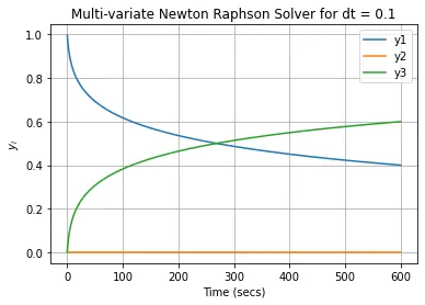
y1 = 0.3999757538866395 y2= 2.6317792810230758e-06 y3 = 0.6000216143340761

The above program and graph solves the three ODE by using the multi variate newton raphsons solver and gives the values of final value of

y1 =0.3999757538866395

y2 = 2.6317792810230758e-06

y3 =0.6000216143340761