Week 3 - External flow simulation over an Ahmed body.

Aim: To simulate the velocity variation across the Ahmed body, using a Steady-state solver with K-epsilon turbulence model in fluent.

The geometry was initially uploaded in space claim and two enclosures were created as shown below

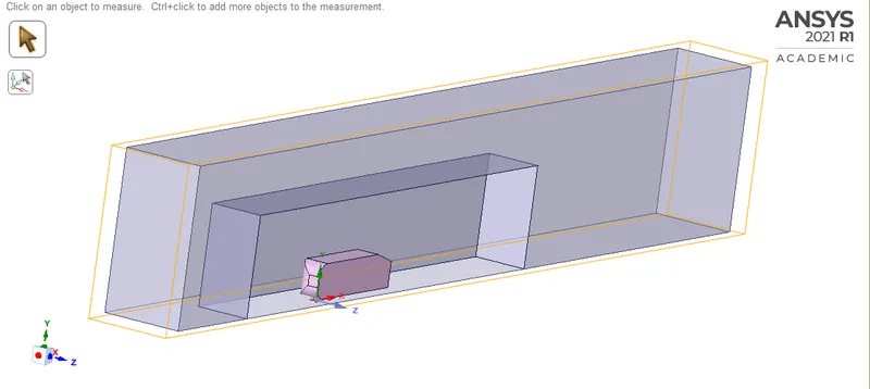
Since the Ahmed body is symmetric, a symmetric plane is used for cutting the body and meshed, by this, we reduce the computational effort, hence faster calculation.

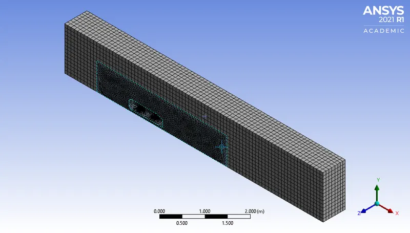
The outer enclosure is created by using hexagonal elements, whereas the inner enclosure tetragonal elements were used, furthermore to capture the drag effects we have used the inflation layers around the Ahmed body and the base below it. The total number of elements was 113281.

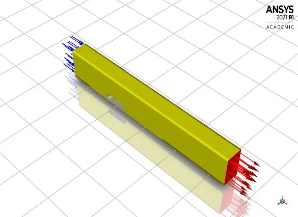
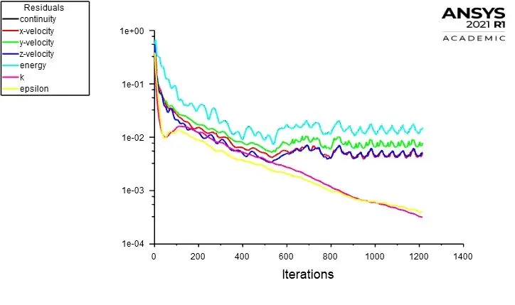
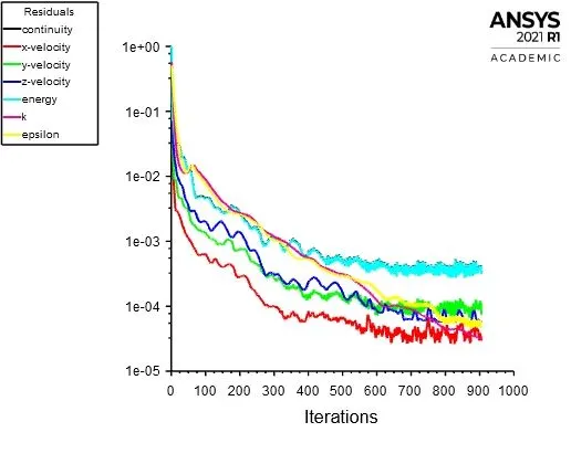
The uploaded mesh into the fluent, has been given the following boundary conditions, inlet velocity of 25 m/s using a density-based solver with k-epsilon turbulence model was solved in the fluent till convergence criteria were observed in the residuals as well as the plots .

What is an Ahmed Body:

S.R. Ahmed first introduced the Ahmed Body in his 1984 paper "Some Salient Features of the Time-Averaged Ground Vehicle Wake." It has since become the gold standard for aerodynamic simulation software. The length of the simple geometrical shape is 1.044 meters, the height is 0.288 meters, and the width is 0.389 meters. It also includes 0.5-meter cylindrical legs attached to the bottom of the body, as well as a 40-degree slope on the back surface.

Formation of the low-pressure region at the wake or trailing end:

The drag-causing eddies (vortices) formed by the pressure difference between the top and bottom of the Ahmed body at the rear trailing end move closer together as the wake area is lowered. As a result of the smaller eddies, less kinetic energy is dissipated, requiring less compensatory power from the engine to move the vehicle forward. As a result, more pressure is applied to the body's rear surface, resulting in less form drag.

Grid Independency test

Mesh	No of Cells	Drag Coefficent	Lift Coefficent
Coarse	113166	0.20449807	0.13014314
Fine	371168	0.20595232	0.1539718

% of variation in drag coefficient = (drag coeff in fine -drag coeff in coarse )/drag coeff in coarse = 0.7%

% of variation in lift coefficient = (lift coeff in fine -lift coeff in coarse )/liftcoeff in coarse = 18.3%

% variation of drag coefficient in comparison with analytical with coarse and finer grids.

coarse grid is 31.8%

finer grid is 31.3% ,

If we compare the variation of finer and coarse grids from the analytical value it appears that the variation between finer and coarser grids is less.Hence we can say that our numerical solution has reached to its reached its rated capacity to predict the analytical solution ,thus further reduction in element size will not affect the value of numerical solution.

Comparison of the velocity contours and vectors with finer and coarse grids:

velocity contours in finer grids velocity contours in coarse grids

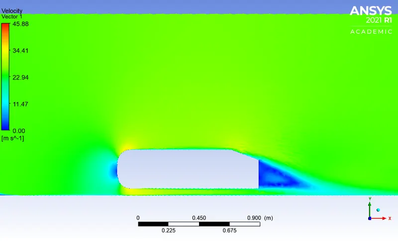
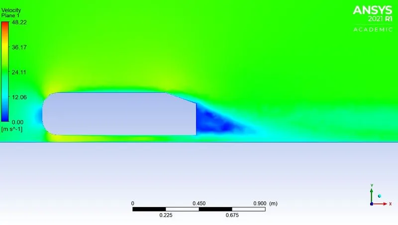
velocity vectors in finer grids velocity vectors in coarse grids

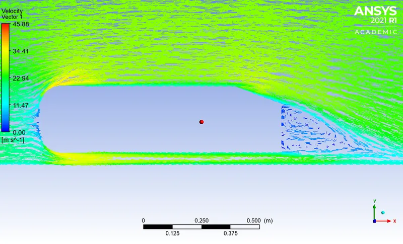
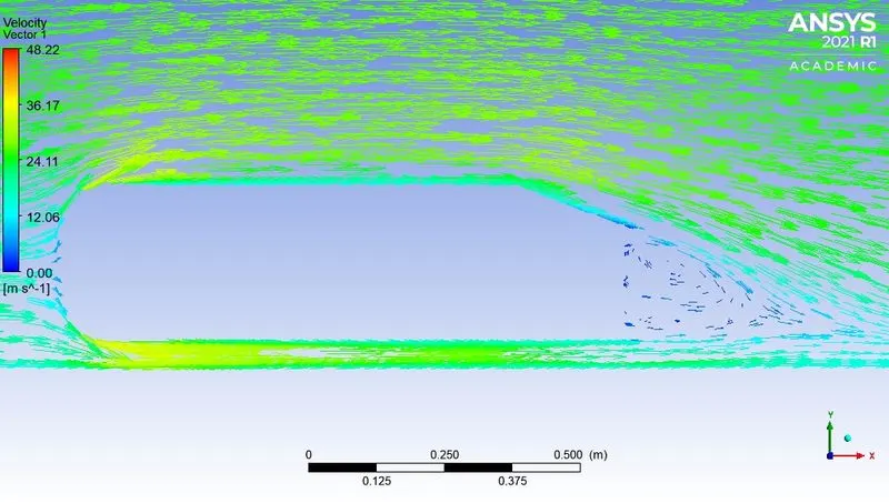
Its observed that , the eddies formation was captured in both the grids, at the wake region. With finer grids the velocity contours are less diffused, moreover, the two eddies formation in the wake region were clearly depicted in the finer grids in comparison with coarse grids.

Coming to contours of the velocity, the low-pressure region behind the wake is less diffused in the case of finer grids, whereas it appears diffused in coarse grids.

Comparison of the pressure contours with finer and coarse grids:

Pressure Contours in finer grids Pressure Contours in coarse grids

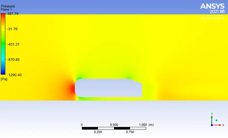
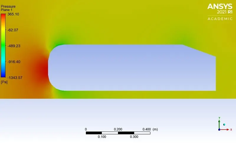
Pressure contours ashows a high-pressure region at the front end and,a low-pressure region was shown at the rear end.

Drag Coefficient and lift coefficient

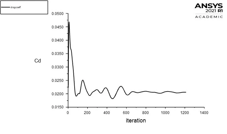
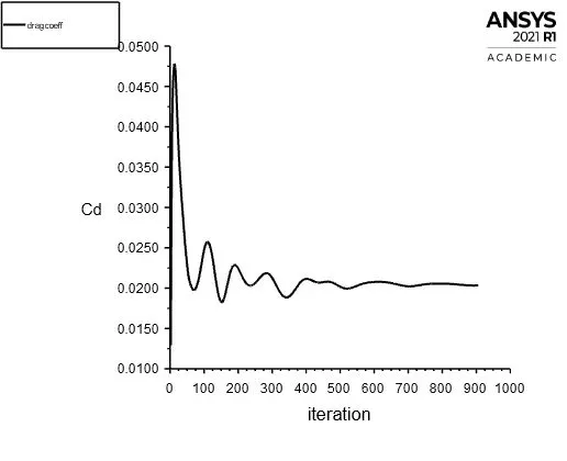
Drag Coefficient in finer grids Drag Coefficient in coarse grids

Lift Coefficient in finer grids Lift Coefficient in coarse grids

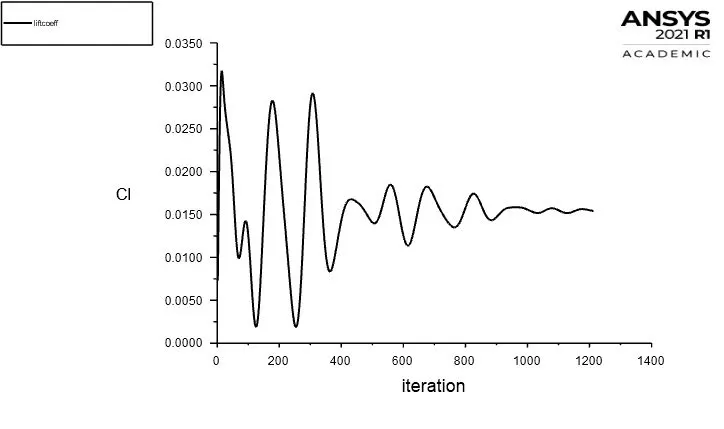
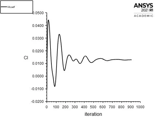
The lift and drag coefficients dont vary after the convergence criteria is reached.

Residuals:

For Coarse grid

For fine grid