Week 5.2 - Literature review: ODE Stability

Aim : To prove the stability condition of ODE , by comparing the analytical solution with explicit and implicit schemes .

Methodology : To prove this we have assumed an ODE

`y' =-100*y-e^t`

where the initial value of this ODE is

`y(0) =0`

that is at time t =0 , y =0

the analytical solution of this ODE is given by

`y(t)=1/99*e^(-100*t)( 1-e^(99*t))`

which will be plotted against time , and compared with numerical solutions of explicit and implicit type

firstly the explicit method , the explicit method utilizes the forward difference scheme , which uses the present time step to predict the future time step , the ODE can rewritten in the FDF as

`(y(t+1)- y(t))/dt =dy/dt =-100*y-e^(-t)`

`(y(t+1) =+y(t)) -(100*y+e^(-t))dt`

similarly we formulate the ODE in implicit method for which we use the bakcward difference scheme , where we use the previous time step to predict the present time step , our ODE in BDF form can be given as

`(y(t)- y(t-1))/dt =dy/dt =-100*y-e^(-t)`

the final form of the equation for y(t) will be

`y(t) = (y(t-1) -e^(-t))*dt /(1+100*t`

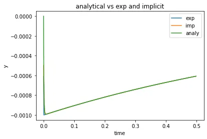
its observed in the below code that all three coincide with each other for the time step of dt =0.001 , and total time of 0.5 , the below code produces the output

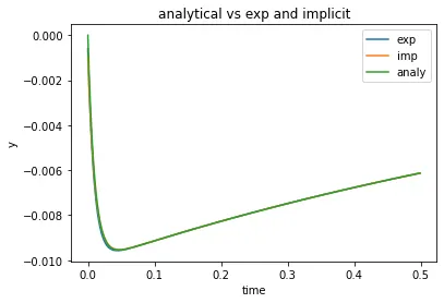
if we increase the time step, the explicit scheme sighlty diverges from the actual and implicit solution and if we still further increase the time step , the explicit solution diverges and becomes unstable,

which is shown below for various time steps for

dt = 0.009 dt = 0.012 dt =0.02

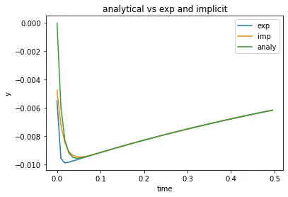
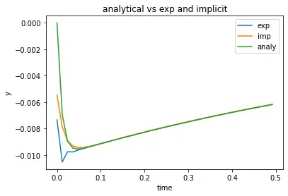
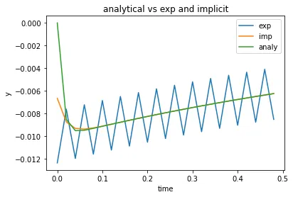
its observed that as we increase the time step the the explicit solution diverges a lot .

Now we repeat the sam method by increasing coefficient value of y in the ODE , to 1000 and observe the same

dt = 0.009 dt = 0.012 dt =0.02

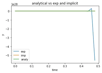
its seen that for higher coefficients of y the solution diverges rapidly in comparison with smaller coefficients

• From the above results following inferences can be made , that is while we are using an ODE in explicit method the ODE is conditionally stable , that is it is succepteble to diverge when we use an higher time step.Where as the implicit scheme doesnt diverge irrespective of the timestep dt
• Stability is an crucial parameter for engineering problems , in solutions which are solved by an explicit method , non dimensional parameter called courant number is kept below 0.5 , else the solution diverges , this is attained by either coarsing of the grid (mesh) or refining the time step.
• Stability of all types of ODE is difficult to predict it is generally seen by increasing the time step gradually and observe when it diverges , and keep the time step accordingly small.

""
Created on Sun Jan 22 11:18:16 2023

@author: Sai krishna kanth
"""
import numpy as np 
import math 
import matplotlib.pyplot as plt


"""
Forward difference method 
explicit scheme , since we are using the known values of present time step 
to calculate the values of future time steps
then our ode can re written as 
(y(t+1) -y(t))/dt = -100*(y)-e^(-t) 
(y(t+1) -y(t)) = (-100*(y)-e^(-t))*dt
y(t+1)  = y(t)+(-100*(y)-e^(-t))*dt
"""
def explicit(t_tot,dt):
   t=np.arange(0,t_tot,dt)
   y = np.zeros(len(t))
   for i in range(0,len(t)):
       y[i] = y[i-1] + dt*(-100*y[i-1]-np.exp(-t[i-1]))
   return [t,y] 
"""
Backward difference method 
implicit scheme , since we are using the unknown values of  present time step 
by using the old values of previous time step
then our ode can re written as
(y(t-1) -y(t))/dt = -100*y(t)-e^(-t) 
(y(t) -y(t-1)) = (100*(t)*y(t)+e^(-t))*dt
-y(t)+(100*(t)*y(t) = y(t-1)-e^(-t))*dt
y(t)(1+100*t) = (y(t-1) -e^(-t))*dt)
y(t) = (y(t-1) -e^(-t))*dt) /(1+100*t) 
"""
def implicit(t_tot,dt):
   t=np.arange(0,t_tot,dt)
   y = np.zeros(len(t))
   for i in range(0,len(t)):
       y[i] = (y[i-1] -np.exp(-t[i])*dt)/(1+100*dt)
   return [t,y]

"""
Analytical  method 
The ODE is integrated such that we get the values of y for 
all the timesteps (t)
 y'=-100*(y)-e^(-t) 
 when y(0) = 0
after integration 
  y(t)=(1/99)*e^(-100*t)*(1-e^(99*t))
 """
def analytical(t_tot,dt):
   t=np.arange(0,t_tot,dt)
   y = np.zeros(len(t))
   for i in range(0,len(t)):
       y[i] = ((1/99)*(math.exp(-100*t[i])))*(1-math.exp(99*t[i]))
   return [t,y]
 
t_tot = 0.5
dt =0.001
t,y_explicit = explicit(t_tot, dt)
t,y_implicit = implicit(t_tot, dt)
t,y_analytical = analytical(t_tot, dt)
plt.plot(t,y_explicit)
plt.plot(t,y_implicit)
plt.plot(t,y_analytical)
plt.xlabel("time")
plt.ylabel("y")
plt.legend(['exp','imp','analy'])
plt.title("analytical vs exp and implicit")

plt.plot
plt.show()