Week 9 - FVM Literature Review

finite volume method :Finite volume method is numerical method of integration , here we divide the domain in finite volumes and calculate the effect of the surfaces of the volume on a central node.

We show the numerical descritization of the finite volume method using an ine dimensional conduction equation with no source term

the equation takes the form

`d/dx(k(dT)/dx) +S =0`

where k is the thermal conductivity and S is the source term

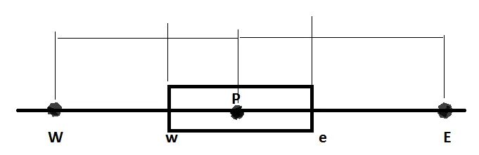
here the domain is discretized into control volumes where the governing equation are solved

W is the node on west side of the central node P ,

E is the node on east side of the central node P.

`deltax` distance between P and W,P and E

w is the face in the west side of the central node P

e is the face in east side of the central node P

w and e are at equal distance of `(deltax)/2` from the central node of the cell

`intd/dx(k(dT)/dx)dV +intSdV =0`

`k_e((dT)/dx)_e - k_w((dT)/dx)_w +s(gradV)` =0

`k_e((T_E-T_P)/(deltax))_e - k_w((T_P-T_W)/(deltax))_w +s(gradV)` =0`

where as the

`k_e = (k_E+K_P)/2`

`k_w = (k_W+k_P)/2`

`S =S_u+ S_pphi_p`

the equation can be re written as

`T_P((k_w.A_w+k_e.A_e)/(deltax) -S_p) = T_W(k_w.A_w)/(deltax) +T_E(k_w.A_w)/(deltax) +S_u`

the above equations can be written in the form as

`a_pT_P=a_wT_W +a_eT_E +S_u`

where

`a_p = a_W+a_E -S_p`

`a_E =k_e.A_e/(deltax)`

`a_W =k_w.A_w/(deltax)`

similar equations are formed for all the nodes, and arranged in the matrix form and the temperature at all the nodes are calculated using gauss elimination techniques.

Major Differences between FDM and FVM

In finite difference method , the taylor series expansion is used for finding the variables at nodes ,

The domain is descritized into nodes , where as the FVM the domain is descritized into finite volumes and on each volume governing equation like conservation of mass , momentum and energy can be solved.

In FDM the domain is descritized into structured grid generally into hexagonal cell, where as unstructured grid can be used in FVM , the efforts for conversion of grid into structired form is reduced.

Interpolation schemes in FVM

Central Difference Scheme:

The value at the faces of the control volume is taken by using the below relations

`T_e =(T_P+T_E)/(2)`

`T_w =(T_P+T_W)/(2)`

Upwind SCHEME:

in an upwind scheme the tempearture at the faces are interpolated as the following

for a positive flow

`T_p=T_e`

`T_w = T_W`

for a flow in negative direction

`T_w = T_P`

`T_e = T_E`

HYBRID SCHEME

In an hybrid scheme is a combination of both upwind and central difference scheme .This can be very useful in solving the convection -diffusion kind of problem , where for Peclet number greater than 2 , the scheme shifts to upwind scheme .

peclet number is calculated at each face of the cell, by using the formula

`Pe =F/(k/(deltax))` = convection /diffusion

when Pe>=2 upwind scheme, -2<=P<2 central differencing scheme

QUICK SCHEME

In this scheme the a quadratic relation is used for finding the temperature at the faces of the cell

`T_(face) = 6/8(T_(i-1)) +3/8(T_(i))-1/8(T_(i-2))`

where i-1 and i-2 are upstream of the node

Flux Limiters

The flux limiters are used in a scheme called total variation diminishion , it helps the scheme to not create new maximum or minimums , so the solution remains in the bounded .This problem arises when we are extrapolating the values of the next cell.

In other words solution doesnot overshoot or undershoot , when we are extrapolting the values of the next cell.