Project 1- Creating your own openFOAM solver

Scalar Transport Equation

For solving the scalar transport equation

`(dels)/(delt)+nabla.(us)=0`

we are using the icoFoam solver

1. Copying the icoFoam solver from the solvers to applications directory

2. Moving the solvers to application directory which i created , and editing the "icoFoam.C" code by using the gedit
"icoFoam.C" or "vim icoFoam.C" command and adding the scalar Transport equation after the piso loop

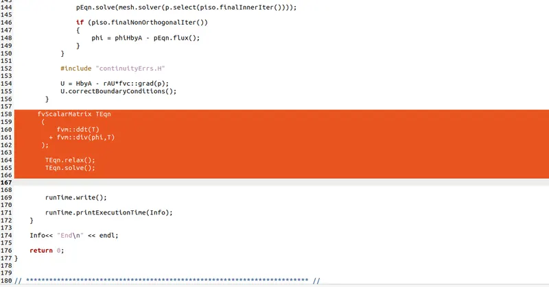
named fvScalarMatric TEqn , where T is the scalar which will be used in this equation,

3. After saving this we will rename this file as scalarFoam.C by using the command

mv icoFoam.C scalarFoam.c

4.Since we have added a new equation which requires temperature, we need to add an IOobject in "createFields.H" ,

gedit createFields.H

and its located in the "0" directory of the case file , as shown below and save it

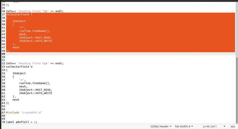
and allowing to auto write after every time step and saving the file

5. Once we have completed this we need to compile this solver, so that we can use it in our cavity case . for compiling we need to access "Make" folder in the solver and edit the files and options

in files

gedit Make/files

scalarFoam.C

EXE = $(FOAM_USER_APPBIN)/scalarFoam

changed the icoFoam.C to scalarFoam.C and the executable location to $(FOAM_USER_APPBIN) instead of $(FOAM_APPBIN) which allows us to store the executable in the user dierctoy and not disturbing the actual executables directory.

now moving to the options directory

gedit Make/options

EXE_INC = \
    -I$(LIB_SRC)/finiteVolume/lnInclude \
    -I$(LIB_SRC)/meshTools/lnInclude

EXE_LIBS = \
    -lfiniteVolume \
    -lmeshTools

which should not be changed, which has location of the "include" files and "library " files

6. Now we are ready to compile this new solver named "scalarFoam" for compiling we need to come out of Make folder and and use wmake command

$> cd..
$> wmake

which compiles teh solver and creates an binary file in $FOAM_USER_APPBIN" folder named "scalarFoam"

7. Now we navigate to "tutorials" by using a shortcut "tut" and copying a case file named cavity which is under incompressible/icoFoam/cavity

and copying it run folder which is $WM_PROJECT_USER_DIR " and renaming it to scalar cavity

8. Now adding the temperature file in 0 folder of scalarCavity case

by adding a file T

/*--------------------------------*- C++ -*----------------------------------*\
| =========                 |                                                 |
| \\      /  F ield         | OpenFOAM: The Open Source CFD Toolbox           |
|  \\    /   O peration     | Version:  v2012                                 |
|   \\  /    A nd           | Website:  www.openfoam.com                      |
|    \\/     M anipulation  |                                                 |
\*---------------------------------------------------------------------------*/
FoamFile
{
    version     2.0;
    format      ascii;
    class       volScalarField;
    object      T;
}
// * * * * * * * * * * * * * * * * * * * * * * * * * * * * * * * * * * * * * //

dimensions      [0 0 1 0 0 0 0];

internalField   uniform 0;

boundaryField
{
    movingWall
    {
        type            zeroGradient;
    }

    fixedWalls
    {
        type            zeroGradient;
    }

    frontAndBack
    {
        type            empty;
    }
}

// ************************************************************************* //

in the "0" directory ,

9. next we need to change the system/controDIct file , to show the type solver we need to use

application     scalarFoam;

instead of

application     icoFoam;

and we need to save it

10. to solve the scalar transport equation we need to add div(phi,T) to the divergence schemes used in "fvSchemes"

divSchemes
{
    default         none;
    div(phi,U)      Gauss linear;
    div(phi,T)      Gauss upwind;
}

and save it

11. in the system fvSolution we need to add the type of solver for temperature

 T
    {
        solver          PBiCGStab;
        preconditioner  DILU;
        tolerance       1e-06;
        relTol          0.05;
    }

    
 TFinal
    {
        $T;
        relTol          0;
    }

12 . Now we are adding a setfields directory to understand the effect of the scalar more clearly

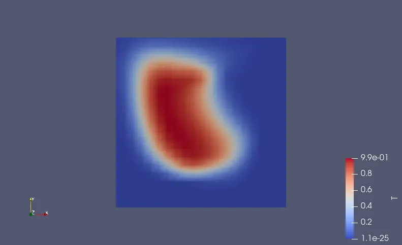
which creates a temperature field initially at the centre and we can observe what is the effect of velocity on it .

FoamFile
{
    version     2.0;
    format      ascii;
    class       dictionary;
    location    "system";
    object      setFieldsDict;
}
// * * * * * * * * * * * * * * * * * * * * * * * * * * * * * * * * * * * * * //

defaultFieldValues
(
    volScalarFieldValue T 0
);

regions
(
    sphereToCell
    {   
        centre (0.05 0.05 0);
        radius 0.03;
        fieldValues
        (
            volScalarFieldValue T 1
        );
    }
);


// ************************************************************************* //

which should be saved it system as setFieldsDict

12. Now we are all set to run the case , firstly generating the mesh by using the blockMesh command , which generates the mesh and now using the solver

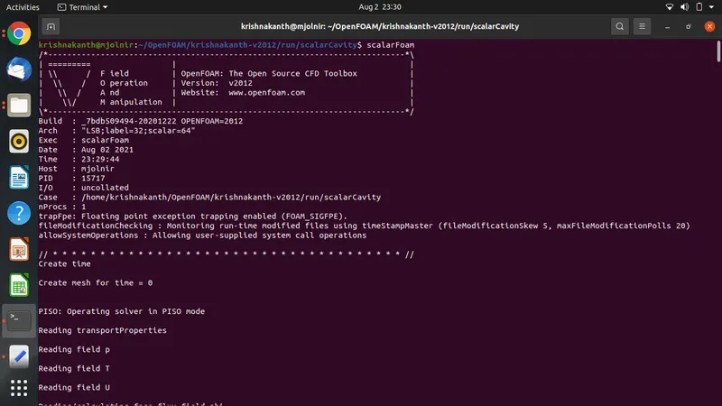
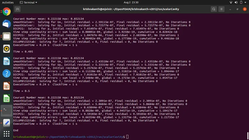
Which sucessfully runs!

13. Now observing the result in paraview , by using the paraFoam command , and seeing the variation from

inital time step

final time step

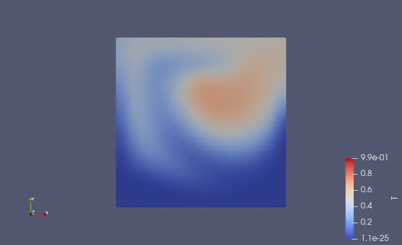
in the final time step we can see that how the scalar quantity has dispersed in the domain due to the presence of the velocity , since we have only considered the advection term , we cannnot observe the diffusion of the scalar in the domain